
ARIMA estimation and short-term forecasting
Part 2 moves from description to forecasting. Since Part 1 showed that Slovenia’s GDP is persistent, seasonal and non-stationary in levels, the natural question is whether a statistical model can use that structure to forecast the near future. The ARIMA model used here is estimated on the transformed series and evaluated over an eight-quarter holdout period. This is a statistical forecasting exercise, not a structural macroeconomic model. It does not explain GDP through consumption, investment, exports, industrial production, fiscal policy or external demand. It asks whether the past behaviour of the series itself contains enough information for short-term projection.
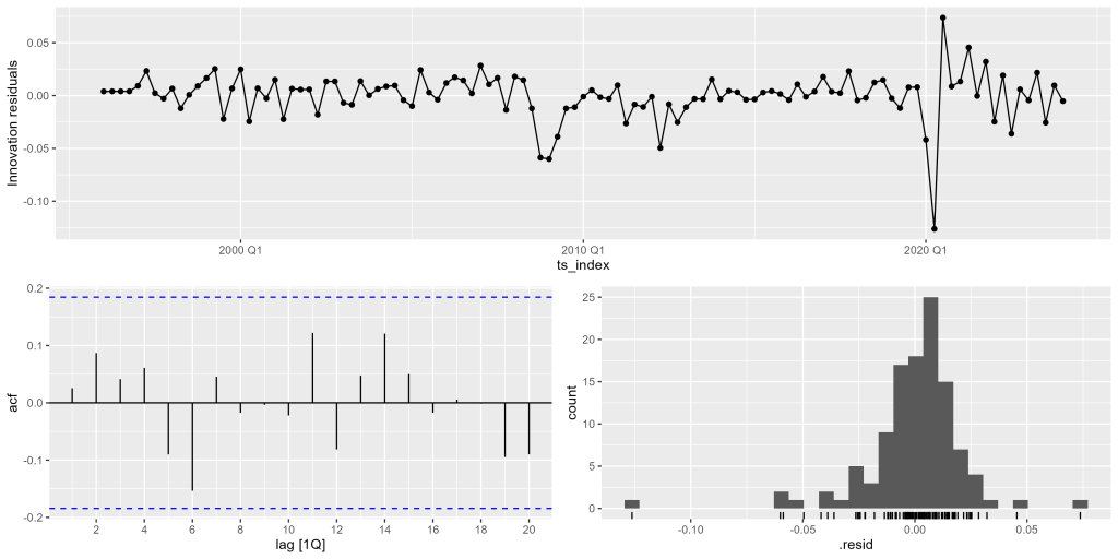
Table 2 reports an ARIMA model with two autoregressive coefficients, one seasonal moving-average coefficient and a positive constant. The first autoregressive coefficient is about 0.714 and is highly statistically significant. The second autoregressive coefficient is about 0.201 and is also statistically significant. Together, these coefficients confirm that Slovenia’s GDP has strong inertia: current movements are meaningfully linked to recent past movements. The seasonal moving-average coefficient is about -0.691 and is highly significant, confirming that seasonal corrections are important in the model. The constant is positive and statistically significant, which is consistent with an underlying growth tendency in the transformed series.
Table 2. ARIMA model estimation and parameters accuracy
| Model | arima | ets | naive | snaive |
|---|---|---|---|---|
| sigma2 | 0.001 | 0.000 | 0.002 | 0.001 |
| log_lik | 258.277 | 166.732 | NA | NA |
| AIC | -506.554 | -315.464 | NA | NA |
| AICc | -505.971 | -313.717 | NA | NA |
| BIC | -493.097 | -290.918 | NA | NA |
| MSE | NA | 0.000 | NA | NA |
| AMSE | NA | 0.001 | NA | NA |
| MAE.x | NA | 0.003 | NA | NA |
| lb_stat | 5.739 | 6.524 | 246.619 | 103.561 |
| lb_pvalue | 0.332 | 0.259 | 0.000 | 0.000 |
| .type | Test | Test | Test | Test |
| ME | -0.017 | -0.022 | 0.058 | 0.019 |
| RMSE | 0.020 | 0.025 | 0.068 | 0.023 |
| MAE.y | 0.017 | 0.022 | 0.060 | 0.021 |
| MPE | -0.364 | -0.459 | 1.218 | 0.399 |
| MAPE | 0.364 | 0.459 | 1.250 | 0.431 |
| ACF1 | -0.236 | -0.344 | -0.382 | 0.349 |
| estimate__ar1 | 0.714 | NA | NA | NA |
| std.error__ar1 | 0.094 | NA | NA | NA |
| statistic__ar1 | 7.624 | NA | NA | NA |
| p.value__ar1 | 0.000 | NA | NA | NA |
| estimate__ar2 | 0.201 | NA | NA | NA |
| std.error__ar2 | 0.095 | NA | NA | NA |
| statistic__ar2 | 2.121 | NA | NA | NA |
| p.value__ar2 | 0.036 | NA | NA | NA |
| estimate__sma1 | -0.691 | NA | NA | NA |
| std.error__sma1 | 0.100 | NA | NA | NA |
| statistic__sma1 | -6.900 | NA | NA | NA |
| p.value__sma1 | 0.000 | NA | NA | NA |
| estimate__constant | 0.002 | NA | NA | NA |
| std.error__constant | 0.001 | NA | NA | NA |
| statistic__constant | 3.493 | NA | NA | NA |
| p.value__constant | 0.001 | NA | NA | NA |
Economically, this model captures three elements: trend-like drift, persistence from the recent past and seasonal correction. The positive autoregressive terms tell us that shocks do not disappear immediately. The negative seasonal moving-average term suggests that seasonal innovations are corrected across comparable quarters. This structure is plausible for a mature European economy whose GDP path is smooth in normal periods but still affected by large shocks.
The residual diagnostics are acceptable. The Ljung-Box p-value for the ARIMA model is about 0.332, so the residual autocorrelation test does not reject the model at conventional significance levels. Figure 4 supports this interpretation. Most residuals fluctuate around zero, though larger disturbances remain visible around the global financial crisis and COVID-19. These events should not be interpreted as ordinary forecasting errors. They are exceptional macroeconomic shocks that a univariate time-series model cannot anticipate from the internal structure of the series alone.
The model comparison in Table 2 favours ARIMA. Its holdout MAPE is about 0.364%, lower than ETS, the naive model and the seasonal naive model. Its RMSE and MAE are also lower than the benchmark alternatives. This matters because a forecasting model should not simply fit the training sample. It should also outperform simple rules such as using the previous value or the same quarter from the previous year. In this case, the ARIMA model provides the strongest short-term statistical benchmark.
Figure 5 and Table 3 show the eight-quarter forecast from 2024Q2 to 2026Q1. The forecast preserves the seasonal profile of the GDP index while projecting continued high levels. All actual holdout observations fall inside both the 80% and 95% prediction intervals. This is a strong practical result. It means that the model’s uncertainty bands are wide enough to contain the realised path, while still remaining analytically informative.
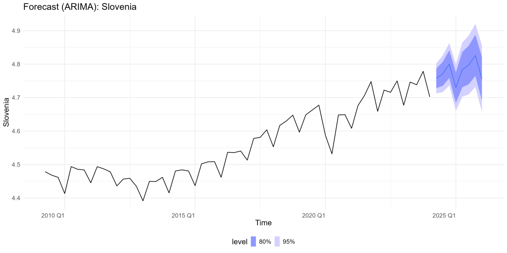
The point forecasts are close to the actual values in several quarters, although the model tends to overpredict slightly during the holdout period. In 2024Q2, the actual value is 116.386 and the forecast mean is 116.444. In 2024Q4, the actual value is 120.877 and the forecast mean is 121.486. In 2025Q4, the actual value is 123.260 and the forecast mean is 124.742. The largest relative gap appears in first-quarter observations such as 2025Q1 and 2026Q1, where actual GDP is below the forecast mean but still within the forecast intervals. This suggests that the model captures the broad level and seasonal structure well, but it may slightly overstate the central path in the latest observations.
Table 3. Forecast eight quarters ahead — ARIMA model
| Date | Actual | Mean | Lower 80% | Upper 80% | Lower 95% | Upper 95% |
|---|---|---|---|---|---|---|
| 2024 Q2 | 116.4 | 116.4 | 113.1 | 119.9 | 111.4 | 121.8 |
| 2024 Q3 | 116.3 | 118.1 | 113.9 | 122.4 | 111.8 | 124.7 |
| 2024 Q4 | 120.9 | 121.5 | 116.6 | 126.6 | 114.0 | 129.4 |
| 2025 Q1 | 109.5 | 113.3 | 108.2 | 118.6 | 105.6 | 121.5 |
| 2025 Q2 | 117.4 | 119.5 | 113.4 | 126.0 | 110.3 | 129.6 |
| 2025 Q3 | 118.5 | 121.2 | 114.4 | 128.4 | 111.0 | 132.4 |
| 2025 Q4 | 123.3 | 124.7 | 117.3 | 132.7 | 113.5 | 137.1 |
| 2026 Q1 | 112.8 | 116.3 | 109.0 | 124.1 | 105.3 | 128.4 |
The practical conclusion is that ARIMA is a credible short-term forecasting tool for Slovenia’s GDP. It performs well diagnostically, outperforms the benchmark models and keeps actual values inside the forecast intervals. Nevertheless, it remains a baseline statistical forecast. If a new external shock, policy change or demand shift occurs, the model will recognise it only after it enters the data. For economic interpretation, the ARIMA forecast should be combined with information about European demand, domestic investment, prices, labour-market conditions and policy developments.
Methodological appendix to Part 2
ARIMA stands for autoregressive integrated moving average. The autoregressive part uses past values, the integrated part uses differencing to handle non-stationarity, and the moving-average part uses past shocks or forecast errors. Seasonal ARIMA models extend this logic to recurring quarterly patterns.
In this exercise, the series is split into a training sample and an eight-quarter holdout sample. The model is estimated on the training data and evaluated on observations not used in estimation. Forecast accuracy is assessed using RMSE, MAE and MAPE. RMSE penalises large errors more heavily, MAE measures average absolute error and MAPE expresses error as a percentage of the observed value. Residual diagnostics, especially the Ljung-Box test, check whether the model has left systematic autocorrelation unexplained. For Slovenia, ARIMA performs well both diagnostically and in the holdout comparison.