

ARIMA estimation and short-term forecasting
Part 2 turns from description to forecasting. Since Part 1 showed that Montenegro’s GDP is highly seasonal and non-stationary in levels, the question is whether an ARIMA model can use this structure to produce a useful short-term forecast. The model is estimated on the transformed series and evaluated against benchmark alternatives. This is a statistical forecasting exercise, not a structural macroeconomic model. It does not explain GDP using tourism, investment, exports, public spending or external demand. It asks whether the past behaviour of the series itself contains enough information for near-term projection.
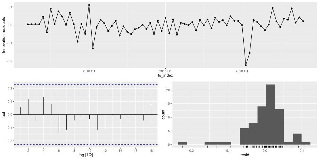
Table 2 reports an ARIMA model with a positive moving-average coefficient of about 0.630, a negative seasonal moving-average coefficient of about -0.687 and a positive constant of about 0.023. All three parameters are statistically significant. Unlike some models for smoother GDP series, this specification does not rely on a reported autoregressive coefficient. Persistence is instead handled through differencing, the moving-average structure and the seasonal component. Economically, this means that the model treats short-run shocks and seasonal corrections as central to Montenegro’s GDP dynamics.
Table 2. ARIMA model estimation and parameters accuracy
| Model | arima | ets | naive | snaive |
|---|---|---|---|---|
| sigma2 | 0.003 | 0.000 | 0.070 | 0.005 |
| log_lik | 102.705 | 49.959 | NA | NA |
| AIC | -197.410 | -81.918 | NA | NA |
| AICc | -196.785 | -79.061 | NA | NA |
| BIC | -188.473 | -61.304 | NA | NA |
| MSE | NA | 0.004 | NA | NA |
| AMSE | NA | 0.004 | NA | NA |
| MAE.x | NA | 0.008 | NA | NA |
| lb_stat | 6.318 | 21.523 | 252.794 | 35.474 |
| lb_pvalue | 0.276 | 0.001 | 0.000 | 0.000 |
| .type | Test | Test | Test | Test |
| ME | 0.050 | 0.008 | 0.245 | 0.038 |
| RMSE | 0.055 | 0.026 | 0.293 | 0.043 |
| MAE.y | 0.050 | 0.023 | 0.245 | 0.038 |
| MPE | 1.012 | 0.156 | 4.888 | 0.777 |
| MAPE | 1.012 | 0.475 | 4.888 | 0.777 |
| ACF1 | 0.028 | 0.086 | -0.040 | 0.165 |
| estimate__ma1 | 0.630 | NA | NA | NA |
| std.error__ma1 | 0.100 | NA | NA | NA |
| statistic__ma1 | 6.282 | NA | NA | NA |
| p.value__ma1 | 0.000 | NA | NA | NA |
| estimate__sma1 | -0.687 | NA | NA | NA |
| std.error__sma1 | 0.141 | NA | NA | NA |
| statistic__sma1 | -4.876 | NA | NA | NA |
| p.value__sma1 | 0.000 | NA | NA | NA |
| estimate__constant | 0.023 | NA | NA | NA |
| std.error__constant | 0.004 | NA | NA | NA |
| statistic__constant | 6.005 | NA | NA | NA |
| p.value__constant | 0.000 | NA | NA | NA |
The positive moving-average coefficient indicates that short-run innovations have a meaningful effect on the following dynamics. The negative seasonal moving-average coefficient is particularly important. It is consistent with the very strong seasonal pattern identified in Part 1 and suggests that seasonal shocks are corrected across comparable quarters. The positive constant captures the upward tendency in the transformed series.
The residual diagnostics are acceptable. The Ljung-Box p-value for the ARIMA model is about 0.276, so the residual autocorrelation test does not reject the model at conventional levels. Figure 4 supports this interpretation. Most residuals fluctuate around zero, but the COVID-19 period appears as a very large negative residual. This is expected. A univariate time-series model cannot anticipate a pandemic collapse using only the internal historical structure of the GDP series. What matters is whether the model captures the regular part of the dynamics after accounting for such exceptional shocks, and the residual diagnostics suggest that it does reasonably well.
The forecast-accuracy comparison is more nuanced than in some other country cases. The ARIMA model has a holdout MAPE of about 1.012%. This is much better than the naive model, but it is worse than the ETS model and also worse than the seasonal naive benchmark. The ETS model has the lowest MAPE in Table 2, around 0.475%, while the seasonal naive model records about 0.777%. This matters. It suggests that for Montenegro, a model that tracks level and seasonality directly may perform better than the ARIMA specification used here. The ARIMA model is statistically coherent, but not the best-performing benchmark in this forecast comparison.
Figure 5 and Table 3 show the forecast path from 2024Q2 to 2026Q1. The forecast preserves Montenegro’s distinctive seasonal pattern: higher values in the third quarter and lower values in the first quarter. This is essential. A model that missed this seasonal rhythm would be unsuitable for Montenegro’s GDP. The forecast intervals are visibly wide enough to reflect the uncertainty created by Montenegro’s strong seasonal and cyclical variation.

The supplied Table 3 reports forecast means and intervals for the forecasting models, but it does not include a separate “Actual” column. For that reason, the exact inclusion of actual holdout values inside the 80% and 95% intervals cannot be verified from Table 3 alone. What can be said from Table 2 is that forecast errors over the holdout period are materially larger for ARIMA than for ETS, and somewhat larger than for the seasonal naive model. The ARIMA forecast is therefore useful as one disciplined benchmark, but not as the preferred single forecasting model for this series.
Table 3. Forecast eight quarters ahead — ARIMA model
| Date | Actual | Mean | Lower 80% | Upper 80% | Lower 95% | Upper 95% |
|---|---|---|---|---|---|---|
| 2024 Q2 | 128.7 | 121.3 | 113.1 | 130.1 | 109.0 | 135.0 |
| 2024 Q3 | 165.3 | 156.0 | 143.7 | 169.5 | 137.5 | 177.0 |
| 2024 Q4 | 136.0 | 129.3 | 119.0 | 140.4 | 113.9 | 146.7 |
| 2025 Q1 | 106.3 | 104.1 | 95.8 | 113.0 | 91.7 | 118.1 |
| 2025 Q2 | 133.9 | 123.0 | 113.0 | 134.0 | 108.0 | 140.2 |
| 2025 Q3 | 172.4 | 159.7 | 146.4 | 174.1 | 139.9 | 182.3 |
| 2025 Q4 | 137.2 | 132.3 | 121.3 | 144.2 | 115.9 | 151.0 |
| 2026 Q1 | 107.9 | 106.5 | 97.7 | 116.1 | 93.3 | 121.6 |
The practical conclusion is that Montenegro’s GDP is forecastable only with caution. Its strong seasonality gives models useful information, but its large shocks and high amplitude make central forecasts fragile. In a small, seasonal economy, a good forecasting workflow should compare several models rather than rely on one specification. ARIMA remains valuable because it formalises differencing, seasonal correction and residual testing. However, in this case, the evidence points to ETS or at least a model-combination approach as a better practical forecasting strategy.
Methodological appendix to Part 2
ARIMA stands for autoregressive integrated moving average. The autoregressive part uses past values, the integrated part uses differencing to handle non-stationarity, and the moving-average part uses past shocks or forecast errors. Seasonal ARIMA models extend this logic to recurring quarterly patterns. In this exercise, the series is split into a training sample and an eight-quarter holdout sample. The model is estimated on the training data and evaluated on observations not used in estimation. Forecast accuracy is assessed using RMSE, MAE and MAPE. RMSE penalises large errors more heavily, MAE measures average absolute error and MAPE expresses error as a percentage of the observed value. Residual diagnostics, especially the Ljung-Box test, check whether the model has left systematic autocorrelation unexplained. For Montenegro, model comparison is particularly important because strong seasonality allows simple seasonal benchmarks to perform well.
