
Part 1. From Post-War Recovery to Mature Expansion
Bosnia and Herzegovina’s GDP as a quarterly time series
Gross domestic product is the broadest single measure of macroeconomic activity. It summarises the value of goods and services produced in an economy and therefore gives a compact view of long-run recovery, expansion, recession and cyclical instability. In this blog post, Bosnia and Herzegovina’s GDP is analysed as a quarterly index, with 2021=100, covering the period from 2000Q1 to 2025Q4. The data source is Eurostat’s quarterly national accounts dataset, namq_10_gdp. Two versions of the series are examined: the original series and the seasonally adjusted series obtained using X13-ARIMA.
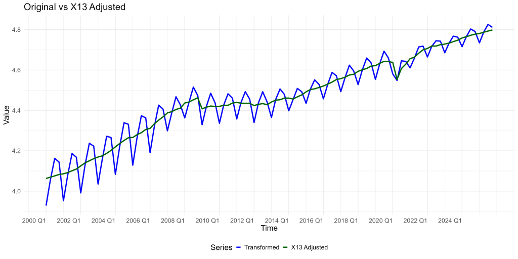
Figure 1 shows a long upward movement in Bosnia and Herzegovina’s GDP. The early 2000s are dominated by recovery and catch-up dynamics. The series rises steadily from a relatively low base, reflecting the long post-war reconstruction and transition process. The mid-2000s bring a visibly stronger expansion, which continues until the global financial crisis. Around 2008–2009, the upward path is interrupted. The fall is not as visually dramatic as the later pandemic shock, but the break in the earlier expansion is clear. After that, the series enters a more moderate growth phase. GDP continues to rise, but the slope is gentler and the path less dynamic.
The COVID-19 shock is clearly visible in 2020. GDP falls sharply, but the decline is short-lived. The rebound that follows is strong, and by the later part of the sample GDP returns to, and then exceeds, its pre-pandemic level. The final observations in 2024–2025 remain high by historical standards, but they do not suggest a new acceleration. The picture is closer to stabilisation at a high level, with some signs of moderation around the trend.
The comparison between the original and seasonally adjusted series is important because quarterly GDP contains regular intra-year movements. These movements can be large enough to obscure the underlying direction of the economy. Seasonal adjustment removes predictable calendar patterns and makes it easier to identify genuine changes in the macroeconomic path. In Figure 1, the seasonally adjusted series provides a cleaner view of trend and cycle, while the original series reminds us that raw quarterly GDP still contains strong seasonal variation.
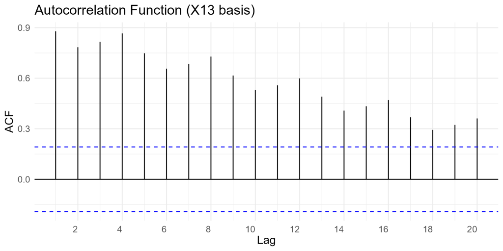
Figures 2 and 3 show how persistent the series is before and after differencing. The autocorrelation function of the log-level series remains strongly positive across many lags. The first autocorrelation is about 0.878, confirming that GDP in one quarter is closely related to GDP in the previous quarter. This is typical for macroeconomic level variables. GDP does not move randomly from quarter to quarter. It reflects accumulated productive capacity, investment, employment, institutions, external demand and policy conditions, all of which evolve gradually.
Figure 3 looks very different. After taking first and seasonal differences of the log series, the autocorrelations become much weaker and mostly remain within the usual confidence bands. The first differenced autocorrelation is slightly negative, around -0.100, while the second-differenced autocorrelation is more negative, around -0.214. This tells us that differencing has removed most of the persistent trend and seasonal structure. The differenced series is therefore more suitable for short-run modelling, while the log-level series is more useful for understanding the long-run macroeconomic path.
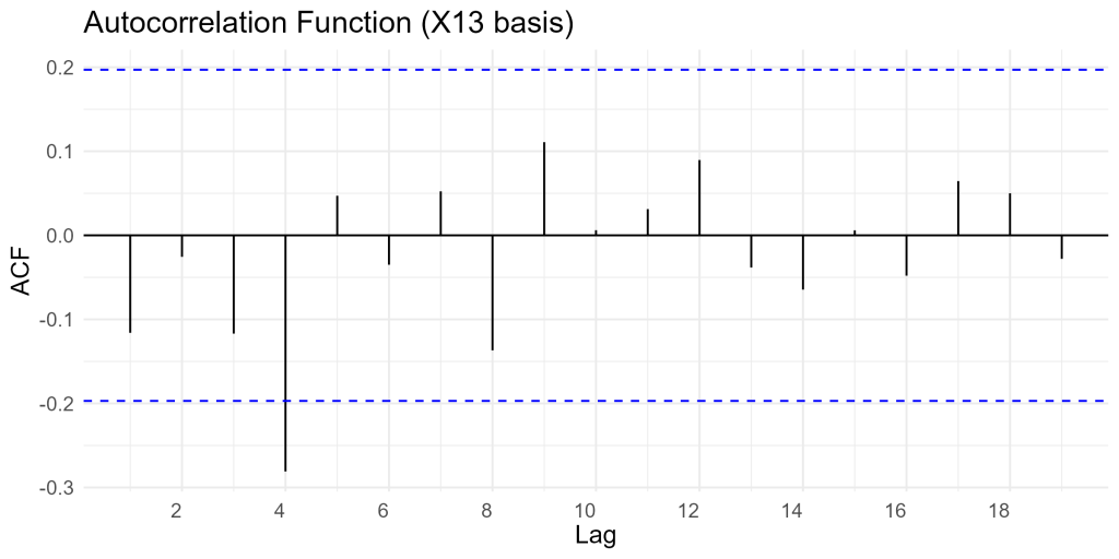
Table 1 reinforces this interpretation. Trend strength is extremely high, around 0.998, which means that the long-run component dominates the series. Seasonal strength is also very high, around 0.977, confirming that seasonal adjustment is essential rather than optional. The seasonal peak is in the third quarter, while the trough is in the first quarter. This is consistent with a quarterly series whose within-year profile is regular and economically meaningful. The spikiness value is very low, suggesting that the series is not driven by random isolated spikes, even though it contains major historical shocks.
Table 1. Features of GDP for Bosnia and Herzegovina time series
| Feature | Value |
|---|---|
| trend_strength | 0.998 |
| seasonal_strength_year | 0.977 |
| seasonal_peak_year | 3 |
| seasonal_trough_year | 1 |
| spikiness | 0.000 |
| linearity | 2.006 |
| curvature | -0.142 |
| stl_e_acf1 | -0.238 |
| stl_e_acf10 | 0.254 |
| acf1 | 0.878 |
| acf10 | 5.452 |
| diff1_acf1 | -0.100 |
| diff1_acf10 | 3.029 |
| diff2_acf1 | -0.214 |
| diff2_acf10 | 2.553 |
| season_acf1 | 0.866 |
| pacf5 | 1.408 |
| diff1_pacf5 | 1.480 |
| diff2_pacf5 | 1.289 |
| season_pacf | 0.312 |
| zero_run_mean | 0.000 |
| nonzero_squared_cv | 0.002 |
| zero_start_prop | 0.000 |
| zero_end_prop | 0.000 |
| lambda_guerrero | 2.000 |
| kpss_stat | 2.067 |
| kpss_pvalue | 0.010 |
| pp_stat | -2.125 |
| pp_pvalue | 0.100 |
| ndiffs | 1 |
| nsdiffs | 1 |
| bp_stat | 80.233 |
| bp_pvalue | 0.000 |
| lb_stat | 82.570 |
| lb_pvalue | 0.000 |
| var_tiled_var | 0.009 |
| var_tiled_mean | 0.933 |
| shift_level_max | 0.150 |
| shift_level_index | 2 |
| shift_var_max | 0.006 |
| shift_var_index | 29 |
| shift_kl_max | 0.174 |
| shift_kl_index | 25 |
| spectral_entropy | 0.182 |
| n_crossing_points | 17 |
| longest_flat_spot | 5 |
| coef_hurst | 0.996 |
| stat_arch_lm | 0.972 |
The linearity measure is positive and relatively large, while curvature is slightly negative. This implies that the long-run path is mostly rising, but not at a constant pace. The residual autocorrelation after STL decomposition is negative at the first lag but positive over longer lags, meaning that some structure remains even after decomposition. The ACF and PACF-based measures show strong persistence in levels and much weaker dependence after differencing. The seasonal autocorrelation remains high, again confirming the importance of the quarterly seasonal pattern.
The stationarity diagnostics point in the same direction. The KPSS statistic is high and its p-value is at the lower bound, which supports treating the level series as non-stationary. The Phillips-Perron result is less restrictive, but the automatic differencing indicators still recommend one ordinary difference and one seasonal difference. The Box-Pierce and Ljung-Box statistics are highly significant in the level series, indicating strong serial dependence before modelling. The variance and shift indicators suggest that the series contains changes in level and variability, with the largest level shift early in the sample and important distributional shifts around the mid-sample. Spectral entropy is low, around 0.182, indicating a structured time-series pattern rather than noise. The Hurst coefficient is close to one, confirming long memory and strong persistence. The ARCH statistic is not large enough to make volatility clustering the central story.
The main conclusion from Part 1 is that Bosnia and Herzegovina’s GDP is a strongly trending, highly seasonal and persistent quarterly series. Its long-run path is one of recovery and expansion, interrupted by the global financial crisis and COVID-19. These features justify the subsequent use of log transformation, seasonal adjustment, differencing and ARIMA modelling.
Methodological appendix to Part 1
The first step in time-series analysis is graphical exploration. Graphs help identify trends, cycles, seasonality, structural breaks, volatility changes and outliers. In quarterly GDP data, the main risk is confusing normal seasonal variation with genuine macroeconomic change. A second risk is over-interpreting one observation without checking whether it belongs to a broader pattern.
The log transformation is used because macroeconomic series often become more variable in absolute terms as their level rises. Logs make changes easier to interpret as approximate percentage movements. First differences focus on short-run change, while seasonal differences compare a quarter with the same quarter in the previous year and help remove recurring seasonal patterns.
The features in Table 1 summarise the behaviour of the series. Trend strength, seasonal strength, autocorrelation, stationarity tests, entropy, spikiness, shift measures and Hurst persistence indicators jointly show whether the series is trending, seasonal, persistent, noisy or structurally unstable. For Bosnia and Herzegovina, they confirm a highly structured, persistent and non-stationary GDP series.