Reading Time: 9 minutes

1. Introduction

Average wages are one of the cleanest windows into an economy’s living-standard dynamics. They condense firm-level conditions, labour-market tightness, bargaining institutions, and macro shocks into a single sequence that households feel directly. In Serbia, wage statistics are published monthly and, viewed over two decades, carry the imprint of several regimes: the pre-GFC expansion, the 2008–09 shock, a long, uneven recovery marked by fiscal consolidation and labour-law changes in the mid-2010s, the pandemic collapse and rebound, and the inflationary surge of 2021–2023. The figures accompanying this post track two closely related nominal series, gross average wages and net average wages, over 2005M1–2025M8, in dinars, and at monthly frequency, using STL for seasonal adjustment and decomposition. Where appropriate, we work with log transformations to stabilise variance; we also examine first differences and seasonal differences to illuminate short-run dynamics. The full set of 13 figures is referenced throughout (Figures 1–13).

Because this is a single-country, multi-series analysis, the narrative compares gross and net wages, highlighting their co-movement and occasional divergence. We emphasise qualitative features visible in the graphs rather than exact point estimates. The goal is to synthesise what the pictures say about Serbia’s income dynamics and to link those patterns to recognisable macroeconomic phases without over-interpreting noise.

At a high level, three features stand out across the period. First, a pronounced long-run upward trend, unsurprising in nominal wages, becomes much clearer once we strip out seasonality. Second, seasonal regularities are visible and persistent, reflecting institutional payment calendars, bonuses, and public-sector disbursement schedules. Third, shock episodes, notably the Global Financial Crisis (GFC) and COVID-19, leave visible departures from trend, with rapid reversals that tell us about the resilience of the underlying labour market. The most recent phase shows a cooling from the post-pandemic surge, with seasonality reasserting itself.

2. Description of the time series and components

2.1 Overall patterns in levels and adjusted series (Figure 1; Figure 2)

The level series display the familiar “staircase” of nominal wages: a rising envelope with month-to-month saw-toothing. Seasonal adjustment compresses the saw-teeth into a smoother trend-cycle, revealing distinct macro phases. In the late 2000s there is a clear interruption consistent with the GFC, followed by a slow normalisation. Around the mid-2010s, the adjusted path becomes steadier, consistent with fiscal consolidation and labour-market reforms, before the abrupt COVID-19 shock and a rapid rebound.

Working in logs (Figure 2) is particularly instructive. The log-transformed series reduce the apparent acceleration that comes purely from nominal base effects, making growth slowdowns and speedups easier to read. In the log scale, the downturns appear as visible level shifts or temporary deviations from a near-linear trend, highlighting two episodes: the 2008–09 downturn and the 2020 pandemic trough. The subsequent period shows an unusually steep segment as nominal wages catch up during the inflation spike, before easing into a more moderate gradient in the last observed year.

Comparing gross and net wages, the co-movement is very tight. Net wages track gross wages with a slightly lower level, as expected, but the amplitude of seasonal movement differs modestly at times, likely reflecting the timing and composition of taxes/contributions, bonuses, and sectoral payouts. During shock episodes, the two series move together; differences in the depth of dips or speed of rebounds are modest and do not persist.

2.2 Main features (Figure 3; Figure 4)

Trend. Decomposition via STL extracts a clear trend component for each series. Over 2005–2025 the trend is upward throughout but with visible breaks in slope during crisis periods. The GFC segment exhibits a trend flattening; the post-2014 stretch is smoother; the pandemic causes a short, sharp deviation with a rapid re-anchoring of the trend line; and the inflationary period produces a temporarily steeper trend that then normalises.

Seasonal. The seasonal component is stable and institutional in character. Monthly wage processes in Serbia often reflect regularities in public-sector payments, year-end bonuses, and firm-level calendars. In the seasonal panels, certain months consistently display peaks or troughs relative to the yearly mean. The amplitude of seasonality changes gradually: it is modest in the mid-2010s relative to the preceding years, then becomes more pronounced during the high-inflation phase as nominal adjustments bunch around specific months.

Irregular. The remainder is generally contained, but outliers coincide with obvious event windows. Pandemic months produce the largest residuals, as one would expect. sharp, idiosyncratic deviations that cannot be explained by the usual seasonal pattern or the smooth trend. Elsewhere, the irregular component is small, suggesting that most month-to-month diversity is seasonal rather than random.

2.3 Brief note on Figure 5 (first and seasonal differences of log series)

In growth-rate form , both gross and net wages are tightly centered around zero, with the seasonally adjusted line (red) lying almost exactly on top of the original (blue).

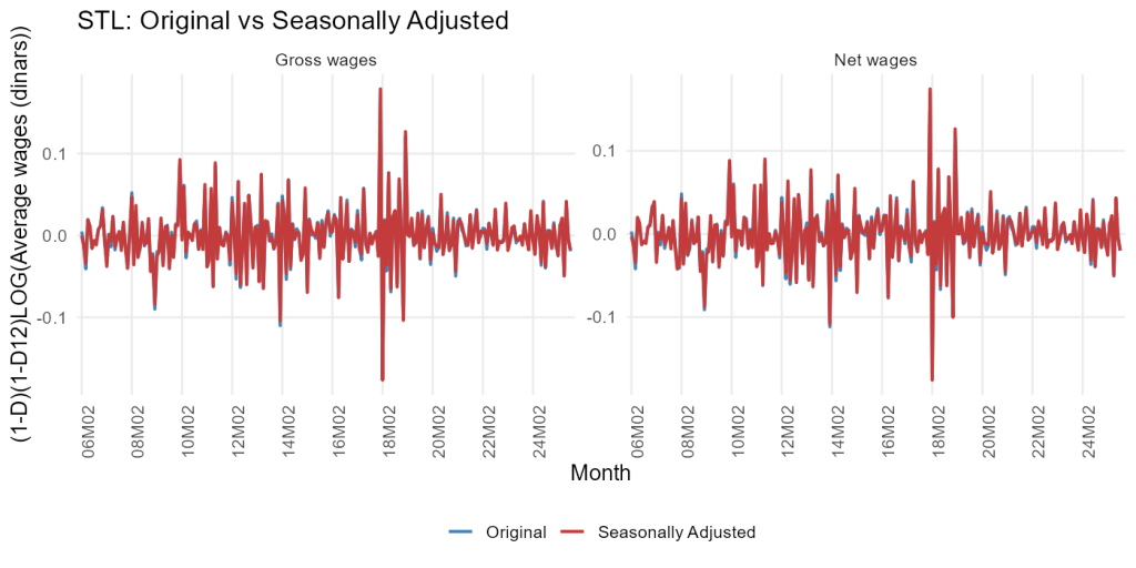
That near-overlap signals that seasonal structure has been effectively removed and that remaining movements are short-run shocks. The series display intermittent volatility bursts, sharp negatives followed by rebounds, most visibly around the major shock windows (GFC and COVID-19), plus a handful of one-off spikes likely tied to administrative or bonus-timing effects. Importantly, the two wage measures behave almost identically in this transformation: no systematic drift, only transitory disturbances, and no evidence of residual seasonality after adjustment.

2.4 Trend vs seasonal dominance and cross-sectional comparisons (Figure 3 & Figure 5 summary)

In a compact summary (trend strength versus seasonal strength), both series lie in the trend-dominant quadrant, consistent with a nominal series driven by inflation and productivity trends, with seasonality as a secondary but persistent feature. The fact that seasonality remains visible even in the presence of a strong trend is important for interpretation: apparent short-term oscillations in levels are mostly calendar effects, not genuine changes in underlying income dynamics.

2.5 Seasonal diagnostics and detailed patterns (Figures 6–13)

The seasonal plots and subseries plots for gross and net wages provide a month-by-month portrait.

The shape of the monthly profiles is stable: particular months are consistently above or below the within-year average. Subseries charts help identify whether those within-year positions drift; there is some evidence of a moderate widening of dispersion in the inflation period, implying that adjustments were less evenly spread through the year.

Lag plots show a strong positive relationship at short lags, unsurprising for a highly persistent series, while also hinting at the seasonal correlation structure at 12-month separations.

The TSstudio seasonal panels (Figures 12–13) add distributional context: month-specific boxplots emphasise medians and dispersion. Months with wider boxes and longer whiskers flag periods where seasonal effects interact with policy or institutional timing, producing larger typical moves and more variability.

Across all diagnostics, the picture is internally consistent. The series are highly persistent, strongly seasonal, and driven by a dominant trend that steepens during high-inflation episodes and flattens during downturns. The gross–net comparison mainly confirms that the tax-contribution wedge shifts levels rather than dynamics, though seasonal amplitude can differ slightly.

3. Economic outlook

The most recent segment of the seasonally adjusted log series points to a normalisation from the post-pandemic–inflation bulge. The steep gradient of 2022–2023 reflects rapid nominal adjustments; by 2024–2025 the slope is more modest, consistent with a disinflation narrative and easing wage indexation pressure. In practical terms, this means the monthly growth in nominal wages has slowed from unusually elevated rates to something closer to pre-pandemic norms, even as the level remains much higher than five years ago.

How should we place Serbia in its regional context? Wage growth across the former Yugoslav region has been shaped by similar forces, tight labour markets, emigration, catch-up, and the global inflation shock. Serbia’s patterns in these figures, sharp but transitory crisis dips, robust rebounds, and persistent seasonality, fit this regional template. Where differences arise, they likely stem from domestic policy timing and sectoral structure: the public sector’s weight, export composition, and the speed of fiscal consolidation can all sharpen or soften seasonal wedges and influence how quickly wages chase prices.

Looking forward, two mechanisms matter. First, labour-market tightness, if vacancies remain high relative to unemployment, wage pressure will persist even as inflation cools. Second, indexation practices, explicit or implicit, shape the timing of pay adjustments and thus the seasonal pattern. If firms revert to spreading adjustments more evenly across the year, we should see a narrowing of month-specific dispersion in the subseries plots; if adjustments continue to bunch, seasonality could remain more pronounced than in the mid-2010s. Either way, the decomposition suggests that the trend dominates: absent a new shock, the main story is a smoother, steadier nominal path.

4. Methodological appendix

4.1 Graphical exploration

Graphs are the first diagnostic in time-series analysis. They reveal trend breaks, seasonal structure, volatility changes, and outliers at a glance, insights that can be obscured in tables. The danger, of course, is over-reading noise or confusing seasonal oscillations with genuine trend changes. That is why this post leans on seasonal adjustment and decomposition before drawing conclusions.

4.2 Transformations (logs and differencing)

When the variability of a series expands as the level rises, a log transformation brings proportional changes into focus and avoids overweighting later years. To inspect short-run dynamics, we also look at first differences and seasonal differences. The former emphasise month-to-month momentum; the latter strip out the recurring 12-month seasonal cycle. These transformations do not “improve” the data per se; they simply allow us to ask different questions of the same underlying process.

4.3 Seasonal adjustment and decomposition using STL

All decompositions in this post use STL (Seasonal-Trend decomposition using Loess). STL iteratively smooths the seasonal and trend components with locally weighted regressions, with a tuning that trades off smoothness and fidelity. It is non-parametric, robust to outliers, and well-suited to monthly data with potentially evolving seasonality. The output is a clean partition of the observed series into trend, seasonal, and remainder, which we then read across episodes. While model-based methods like X-13ARIMA-SEATS or TRAMO/SEATS can be advantageous for calendar effects and forecast-consistent decompositions, STL is an excellent exploratory baseline: transparent, flexible, and easy to replicate.

4.4 Alternative approaches and pros/cons

Had we used a model-based method, we would integrate regression pre-adjustments (e.g., trading-day effects) and explicit ARIMA structures that yield signal-extracted components. The trade-off is complexity and specification risk. In the current application, with two highly persistent nominal series and a focus on visual phases rather than precise seasonal-adjustment benchmarking, STL offers the right balance of robustness and interpretability.

5. Conclusion

From 2005 to 2025, Serbia’s gross and net average wages trace a story of steady nominal ascent punctuated by crises, with seasonality that is distinctive but stable. Decomposition shows that the trend is the main driver, bending during global shocks and steepening during the inflation surge, while seasonal regularities reflect institutional calendars rather than changing fundamentals. The irregular component is usually small, spiking only when the economy is forced off its normal trajectory.

Comparing gross and net wages confirms that the tax-contribution wedge shifts levels but not the skeleton of dynamics. Where differences in seasonal amplitude occur, they are small and episodic. The latest panels indicate a return to normalisation after the extraordinary pandemic-inflation sequence: the slope of the adjusted log series has moderated, and seasonal patterns look more like their mid-2010s selves.

For policymakers and analysts, three implications follow. First, month-to-month noise in nominal wages is mostly seasonal, so policy should be guided by adjusted signals and medium-run trends. Second, the speed of nominal adjustment during inflation shocks is visible in the steepening of the trend; as disinflation proceeds, we should expect, and indeed already see, a gentler profile. Third, monitoring whether seasonal dispersion tightens again will provide early evidence on the re-timing of wage-setting behaviour.

The same framework can be extended easily to real wages, industrial production, or tourism indicators. The combination of log transforms, differences, and STL gives a compact, replicable toolkit for turning raw monthly data into an economic narrative that is at once intuitive and empirically disciplined.

References

Cleveland, R. B., Cleveland, W. S., McRae, J. E., & Terpenning, I. (1990). STL: A seasonal-trend decomposition procedure based on Loess. Journal of Official Statistics, 6(1), 3–73. https://www.math.unm.edu/~lil/Stat581/STL.pdf

Hyndman, R. J., & Athanasopoulos, G. (2025). Forecasting: Principles and practice (3rd ed.). OTexts. https://otexts.com/fpp3

U.S. Census Bureau. (2023). X-13ARIMA-SEATS Seasonal Adjustment Program: Program documentation.

Statistical Office of the Republic of Serbia. Monthly wages (data source for Figures 1–13).

Figures referenced: 1–13 (Original vs SA in levels and logs; STL decompositions; differences diagnostics; seasonal plots; subseries; lag plots; TSstudio seasonal panels). The article relies on qualitative readings visible in those figures and does not impute precise numerical values not shown in the charts.