1. Introduction
Real gross domestic product is the standard yardstick for measuring the scale of economic activity. In the case of Montenegro, quarterly real GDP is compiled as chain-linked volumes with 2020 set to 100, so changes in the index capture movements in the quantity of goods and services produced, net of inflation. For a very small, highly open and tourism-dependent economy such as Montenegro, this series provides a compact narrative of how output has responded to booms in foreign demand, domestic reforms, and large external shocks.
The ten figures that accompany this article show Montenegro’s real GDP from 2006Q1 to 2025Q2 in a variety of perspectives: in logarithms, with and without seasonal adjustment; decomposed into trend, seasonal and irregular components; and transformed into growth-rate form through first and seasonal differencing, again accompanied by decomposition and detailed seasonal diagnostics. Because the variance of the series increases with its level, the analysis works throughout with logs and their differences; equal vertical distances on these plots correspond roughly to equal percentage changes in GDP.
The sample begins shortly before Montenegro’s 2006 independence referendum and spans its subsequent journey as a euroised micro-state and EU candidate country. The country has used the euro as de facto legal tender since 2002, without being a member of either the European Union or the euro area. Over this period Montenegro’s growth model has been dominated by tourism and construction. Official and analytical sources consistently estimate that tourism directly and indirectly generates around a quarter to a third of GDP, and even more of export receipts. This structural feature leaves a clear imprint on the time series: GDP is extremely seasonal, surging in the summer quarters and easing in the winter, with major global shocks transmitting strongly into the domestic cycle.
A high-level comparison between the most recent observations and earlier phases immediately highlights three episodes. The first is the pre-global-financial-crisis boom of 2006–2008, when the seasonally adjusted series rises steeply as foreign capital, tourism and real-estate development fuel rapid expansion. The second is the interruption and partial reversal of that boom during and after the 2008–2009 crisis, when the trend flattens and volatility increases. The third is the extraordinary collapse of activity in 2020 followed by a spectacular rebound in 2021–2022. International data show that Montenegro suffered one of the deepest GDP contractions in Europe in 2020 and one of the strongest rebounds in 2021, reflecting the near-shutdown and subsequent reopening of international tourism. By 2025Q2, the level of seasonally adjusted real GDP is clearly above its pre-COVID peak, but the graphs also suggest a more volatile environment than in the mid-2000s.
2. Description of the time series and components
2.1 Overall patterns in levels and adjusted series
Figure 1 plots the logarithm of Montenegro’s real GDP alongside its STL-based seasonally adjusted counterpart. The unadjusted series traces out the extreme intra-year rhythm of the economy: low activity in the first quarter, a gradual build-up in the second, a very pronounced peak in the third quarter driven by the tourism season, and a substantial step down in the fourth. This pattern is visible from the first year of the sample and becomes even more pronounced over time, with summer peaks rising higher relative to winter troughs.

The seasonally adjusted series removes this regular pattern and reveals the underlying business cycle more clearly. From 2006 to 2008, the adjusted line climbs steeply, capturing the investment and tourism boom that followed independence and euroisation. The global financial crisis interrupts this trajectory: output drops around 2009, and in the early 2010s the adjusted series exhibits a more uneven, stop-go pattern, with short expansions followed by setbacks. These fluctuations reflect a combination of domestic imbalances, the euro-area sovereign-debt crisis and Montenegro’s exposure to foreign funding conditions.
From the mid-2010s until 2019, the adjusted GDP series resumes an upward course, though with more pronounced quarter-to-quarter noise than in the early boom. Tourism continues to expand, large infrastructure projects are launched and negotiated EU accession advances, supporting confidence and investment. The defining break in the series comes in 2020. Both the original and adjusted logs show an unprecedented drop as international travel collapses during the COVID-19 pandemic. The decline is much sharper than in larger, more diversified regional economies, mirroring Montenegro’s extreme reliance on foreign visitors. In subsequent quarters the series rebounds sharply, with seasonally adjusted GDP rising at a pace rarely seen before. By 2022–2023 the level has regained and then surpassed its pre-pandemic peak, albeit with continued volatility as global conditions remain unsettled.
The final part of the sample, up to 2025Q2, suggests that growth has normalised to more moderate rates, but with larger short-run swings than in the pre-crisis period. This pattern captures the tension between strong structural drivers, tourism demand, EU accession prospects and political stability, and vulnerabilities linked to external shocks, energy prices and climate-related risks for coastal tourism.
2.2 Main features: trend, seasonal and irregular components
Figure 2 presents the STL decomposition of the log GDP series into trend, seasonal and irregular components. The trend component provides a smoothed view of Montenegro’s medium-term trajectory. It rises steeply in the years immediately before and after independence, reflecting rapid growth from a low base. It then flattens in the early 2010s, signaling a slowdown after the global financial crisis and amid euro-area turbulence. After about 2015 the trend turns upward again, though with occasional pauses, indicating resumed convergence towards higher income levels. The COVID-19 shock appears as a sharp downward dent in the trend around 2020, followed by an equally sharp upward correction; the decomposition attributes part of the pandemic collapse to irregular movements, but the depth and persistence of the shock are sufficient to leave a visible mark on the medium-term component as well.

The seasonal component is striking. Its amplitude is large relative to the trend, with recurring peaks in the third quarter and troughs in the first, consistent with Montenegro’s economy being one of the most tourism-intensive in Europe. Over the sample, the gap between the typical summer high and winter low appears to widen somewhat, signalling that tourism’s contribution to GDP has grown over time. This is consistent with external estimates that tourism accounts for around 25–30% of GDP and an even larger share of employment and exports. The shape of the seasonal pattern remains broadly stable, however: there is no obvious structural change in the month or quarter of the peak, suggesting that the tourist season has lengthened only gradually, if at all.
The irregular component captures idiosyncratic movements that are not well explained by the smooth trend or regular seasonality. For much of the sample, this remainder is relatively modest, with positive and negative deviations that resemble noise. There are, however, clusters of larger residuals in periods of stress. The quarters around the global financial crisis show noticeable irregular shocks, reflecting sudden stops in capital flows and swings in construction and real-estate activity. The most dramatic spikes in the irregular component occur in 2020 and 2021, underscoring how extraordinary the COVID-19 episode was from a time-series perspective: even after accounting for a shift in trend and the usual seasonal trough, the remaining shock is exceptionally large.
Overall, the decomposition underscores that Montenegro’s GDP dynamics are shaped by three interacting forces: a trend that reflects convergence and crisis-related disruptions; an unusually strong and persistent seasonal pattern tied to tourism; and rare but very large irregular shocks when global crises strike.
2.3 Seasonal diagnostics and detailed patterns
The seasonal diagnostics deepen this picture. The seasonal plot for the log series in Figure 3 displays each observation by quarter, allowing a comparison of the within-year profile over time.

First quarters cluster at the lower end of the distribution; second quarters show intermediate values; third quarters populate the upper tail; and fourth quarters lie between the summer peak and winter low. Over the years the third-quarter observations drift upwards more than those in other quarters, indicating that the expansion has been driven disproportionately by the high season. This is consistent with anecdotal and survey evidence of booming summer tourism and relatively modest growth in the rest of the year.
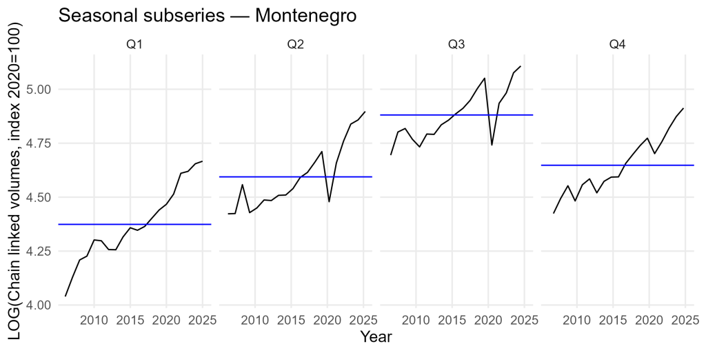
The seasonal subseries plot in Figure 4 tracks each quarter’s path across years as its own mini-series. The first-quarter line rises gently, suggesting gradual strengthening of the non-tourism base, public services, some industry and domestic demand. The third-quarter line slopes more steeply and exhibits larger swings, recording the boom-bust ebb of tourist arrivals and spending. Crisis years, particularly 2009 and 2020, manifest as deep drops in the third-quarter subseries, when the season that normally carries the economy instead collapses.

Lag plots for the log series in Figure 5 show each quarter’s GDP against its lagged value. The points form a tight cluster along a positively sloped diagonal, confirming strong persistence: high output in one quarter tends to be followed by high output in the next, and low output by low output. There is also some curvature and dispersion, hinting at cyclical dynamics and the influence of shocks. Clusters of points corresponding to crisis periods sit noticeably below the main cloud, making clear how unusual those episodes are relative to the economy’s normal autoregressive behaviour.

The diagnostics for the first-differenced logs in Figures 6 to 8 provide a complementary view in growth-rate space. Seasonal plots of the differenced series show systematic differences between quarters, indicating that differencing has not removed the deterministic seasonal pattern. Growth is more volatile in the summer quarters, and winter often delivers small negative or weakly positive growth, even when the annual trend is favourable.
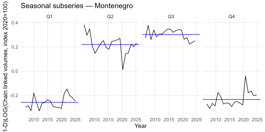
Subseries plots for the differenced series highlight years in which particular quarters deviate strongly from their historical ranges; 2020 again stands out, with unprecedented negative growth across multiple quarters.

Lag plots of the differenced series still show moderate positive autocorrelation, but the relationship is weaker than in levels and more centred around zero, as expected for growth rates.
2.4 Differenced series and decomposition
Figures 9 and 10 focus on the first-differenced log series, which approximate quarterly growth rates. When the series is transformed in this way, the long-run trend disappears and the graph oscillates around zero, highlighting periods of acceleration and deceleration rather than changes in level.

In Figure 9, the original differenced series shows a dense cloud of moderate fluctuations punctuated by a few extreme movements. The global financial crisis appears as a sequence of negative growth quarters clustered around 2009–2010, followed by uneven, sometimes negative growth in the early 2010s. The most striking pattern is the pair of large swings around 2020–2021: a collapse in growth when the pandemic hits, followed by very high positive growth rates as tourism resumes and policy support kicks in. Seasonally adjusting the differenced series reduces some of the intra-year noise, but the major crisis-related swings remain clearly visible.

The STL decomposition of the differenced series in Figure 10 confirms that, once trend is removed from growth rates, the residual component is relatively small in normal times but explodes during crises. The seasonal component of the differenced series is modest but not negligible, indicating that even growth rates retain some seasonal structure, most notably, the tendency for summer quarters to deliver outsized positive or negative surprises relative to the rest of the year. The trend in growth rates hovers close to zero over the long run, consistent with the notion that growth itself does not follow a deterministic linear trend once we look at changes in logs. Instead, the medium-term behaviour of growth is shaped by cycles of expansion and consolidation and by the timing of major shocks.
3. Economic outlook
The recent portion of the series, from roughly 2022 onward, reflects both the resilience and fragility of Montenegro’s growth model. After the historic contraction in 2020, real GDP rebounds strongly, and by 2023–2024 the trend and seasonally adjusted levels are clearly above pre-pandemic benchmarks. Official data indicate that real GDP growth has been robust in these years, with output nearly doubling in euro terms between 2020 and 2024 as tourism, construction and private consumption recover. The time-series graphs show this as a steep upward segment in the trend and a series of large positive growth-rate observations after the trough.
Yet the same graphs underscore how dependent this performance is on external demand and favourable conditions. The sheer amplitude of the seasonal component and the size of the irregular shocks during crises suggest that Montenegro’s GDP will remain highly sensitive to swings in tourism, global financial conditions and geopolitical developments. The country’s unilateral euroisation removes exchange-rate risk and helps anchor inflation expectations, but it also limits monetary-policy autonomy and imposes discipline on fiscal policy in an environment of high import dependence and large current-account deficits.
From a regional perspective, Montenegro behaves like an extreme version of the southern European and Western Balkan tourism economies. It shares with Croatia, Greece and others a strong summer season, exposure to climate-related and geopolitical risks affecting travel, and dependence on the euro area business cycle. But as a very small economy with a narrow productive base, its GDP series is more volatile: the same external shocks that produce noticeable dents in larger neighbours generate deep troughs and soaring peaks in Montenegro’s time series.
Looking ahead to the rest of the decade, the decomposition suggests two broad messages. First, the underlying trend has resumed an upward path, indicating that, barring new crises, Montenegro is again on a convergence trajectory towards higher income levels. Second, the persistent strength of seasonality and the historical size of irregular shocks point to continued vulnerability. Successfully managing this trade-off, leveraging tourism and foreign investment while broadening the economy and strengthening resilience, will determine whether the GDP series in the next twenty years looks smoother than in the past twenty.
4. Methodological appendix
4.1 Graphical exploration
The analysis in this article relies heavily on graphical methods. Simple time-series plots of log real GDP and its seasonal adjustments reveal trends, turning points and changes in volatility. Decomposition graphs separate the long-run trend, the regular intra-year pattern and the residual irregular movements, making it easier to attribute observed fluctuations to structural forces, seasonality or shocks. Seasonal plots and subseries plots display how each quarter behaves across years and within years, while lag plots provide an intuitive visualisation of persistence by showing how current values relate to lagged ones. Used together, these tools help to avoid misreading temporary seasonal fluctuations as trend changes and to detect genuinely unusual observations that may warrant economic interpretation or data quality checks.
4.2 Transformations: logs and differencing
Before decomposition, Montenegro’s real GDP index is transformed by taking natural logarithms. For a series whose fluctuations grow in absolute size as the level rises, this stabilises the variance and puts proportional changes on a roughly comparable scale over time. If ( ) denotes the original index, the log-transformed series is (
 ). The first difference (
 ) approximates the quarter-on-quarter growth rate, while the seasonal difference (
 ) captures year-on-year growth at a quarterly frequency, where the seasonal period (
 ) equals four. By working with these differences, the analysis removes much of the long-run persistence, allowing attention to focus on short-run dynamics and shocks.
4.3 Seasonal adjustment and decomposition using STL
Seasonal adjustment and decomposition are carried out using STL, which stands for Seasonal-Trend decomposition using Loess. Developed by Cleveland and co-authors, STL represents the observed log GDP ( ) is expressed as the sum of three components:
 ,
,
where ( ) is the trend-cycle, (
 ) the seasonal component and (
 ) the irregular remainder. STL estimates these components iteratively. It applies local regression (Loess) over the seasonal cycle to extract a flexible seasonal pattern, then smooths the remaining series over longer windows to obtain the trend, and finally defines the irregular component as what is left over. The procedure is robust to outliers and allows the analyst to choose how smooth the trend and seasonal components should be, making it well suited to series like Montenegro’s GDP that combine strong seasonality with occasional large shocks.
In this application, STL is applied both to the log levels and to the first- and seasonal-differenced logs. In the former case, the goal is to identify the medium-term path of GDP and the shape and strength of its seasonal cycle. In the latter, the focus shifts to growth dynamics: whether any predictable seasonal structure remains in growth rates and how large the irregular shocks are once trend and seasonality have been removed.
5. Conclusion
The ten-figure exploration of Montenegro’s quarterly real GDP from 2006Q1 to 2025Q2 paints the picture of a small, highly open, tourism-driven economy subject to large external shocks. The STL decomposition of the log series shows a trend that climbs steeply before the global financial crisis, flattens during a prolonged adjustment period, and then resumes its ascent in the run-up to the pandemic and again in the post-COVID recovery. The seasonal component is among the strongest in the region, with a towering summer peak that has grown over time, underscoring the economy’s reliance on tourism and related services. The irregular component is modest in normal years but dominates the series during crises, particularly in 2020–2021.
The seasonal diagnostics and the analysis of differenced series confirm these impressions. Growth rates exhibit substantial volatility, especially in the peak season, and are strongly affected by global shocks. At the same time, the latest data show that Montenegro has managed not only to recoup the output lost during the pandemic but also to push GDP to new highs, suggesting a degree of resilience and adaptability.
The challenge for policymakers and investors is to build on this momentum while reducing vulnerability. From a time-series perspective, a more diversified, less seasonal growth model would show up as a trend component that continues to rise, a seasonal component whose amplitude gradually shrinks, and an irregular component that remains small even when the global environment is turbulent. The methods used here, log transformations, differencing, STL decomposition and graphical diagnostics, offer a transparent and replicable way to monitor these developments and can readily be applied to other macroeconomic indicators for Montenegro and its regional peers.
References
Cleveland, R. B., Cleveland, W. S., McRae, J. E., & Terpenning, I. (1990). STL: A seasonal-trend decomposition procedure based on Loess. Journal of Official Statistics, 6(1), 3–73. https://www.math.unm.edu/~lil/Stat581/STL.pdf
Eurostat. (2025). National accounts and GDP – Statistics explained. European Commission. https://ec.europa.eu/eurostat/statistics-explained/index.php/National_accounts_and_GDP
Eurostat. (2024). Gross domestic product (GDP) and main components (output, expenditure and income), quarterly – Chain linked volumes, index 2020 = 100 (namq_10_gdp). Retrieved from Eurostat database.
European Commission. (2025). Montenegro 2025 report. Brussels: Directorate-General for Trade. https://enlargement.ec.europa.eu/document/download/9ae69ea7-81d6-4d6a-a204-bd32a379d51d_en?filename=montenegro-report-2025.pdf
Hyndman, R. J., & Athanasopoulos, G. (2025). Forecasting: Principles and practice (3rd ed.). OTexts. https://otexts.com/fpp3
Vienna Institute for International Economic Studies. (2020). Montenegro: Tourism decline drives major slump in economic growth. wiiw Country Report. https://wiiw.ac.at/montenegro-tourism-decline-drives-major-slump-in-economic-growth-dlp-5462.pdf