1. Introduction
Real gross domestic product is the central summary indicator of economic activity. Measured here as chain-linked volumes with 2020 set to 100, quarterly real GDP for Croatia tracks the evolution of the country’s production of goods and services after stripping out the effect of inflation. It therefore provides a compact view of how the Croatian economy has expanded, contracted and rebalanced over the past quarter of a century. The ten graphs that accompany this article present the series in both level and growth-rate form, decomposed into trend, seasonal and irregular components and supported by a rich set of seasonal diagnostics.
The sample from 2000Q1 to 2025Q2 spans several distinct regimes. Croatia entered the 2000s as a small open economy still consolidating its transition from socialism and the legacy of the 1990s conflict. It then experienced a strong pre-crisis expansion, a deep and unusually prolonged post-2008 recession, gradual recovery in the run-up to European Union membership in 2013, and a tourism-driven upswing in the late 2010s. More recently the series captures the dramatic collapse in activity during the COVID-19 pandemic and the subsequent rebound, culminating in Croatia’s adoption of the euro on 1 January 2023.
Because the variance of GDP tends to rise with its level, the analysis works with logarithms of the index rather than raw values. In that scale, equal vertical distances correspond roughly to equal percentage changes, which makes the growth performance more interpretable over long spans. Seasonal adjustment and decomposition are carried out using the STL procedure (Seasonal–Trend decomposition by Loess), which splits the observed series into a slowly moving trend–cycle, a within-year seasonal pattern and a residual or irregular component.
A useful starting point is to compare the most recent observations with earlier phases. By 2025Q2, the level of seasonally adjusted real GDP is clearly above its pre-global-financial-crisis peak, confirming that the economy has not only made up the ground lost in the 2009–2014 recession but has also recovered from the COVID-19 shock. The post-pandemic rebound is visible as a sharp V-shaped pattern, especially when expressed in growth-rate form. At the same time, the graphs suggest that volatility has not fully returned to its pre-crisis calm; quarterly GDP remains sensitive to tourism, global demand and energy prices, and the series does not settle into a perfectly smooth expansion.
2. Description of the time series and components
2.1 Overall patterns in levels and adjusted series
Figure 1 plots the original and STL-adjusted logarithm of Croatia’s real GDP. The original series displays pronounced intra-year swings, reflecting the familiar rhythm of the Croatian economy: weak activity in the winter quarters, a pick-up in spring, a powerful summer peak driven by tourism and related services, and a cooling in the final quarter of the year. The seasonally adjusted series strips out this regular pattern and reveals a smoother trajectory that is easier to align with macroeconomic events.
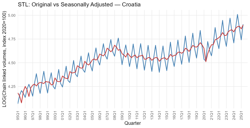
Viewed in this way, the early 2000s are characterised by a steady upward trend, with only modest short-run noise. Real GDP grows almost monotonically until 2008, mirroring a global credit-fuelled expansion and strong capital inflows to emerging Europe. The trend then turns sharply downward during the global financial crisis. The seasonally adjusted line shows not just a one-off drop in 2009 but a multi-year period of stagnation and mild contraction extending well into the first half of the 2010s, consistent with Croatia’s well-documented “double-dip” recession.
EU accession in mid-2013 falls squarely within this period of subdued activity. Rather than a discrete break, the graphs suggest a gradual turning point: the trend stops falling and begins a slow, hesitant ascent. There is no single quarter in which GDP suddenly jumps because of membership; instead, the benefits of improved market access and investor confidence seem to accumulate over several years.
From around 2015 onwards, the seasonally adjusted path steepens. The late 2010s show a sustained expansion, supported by tourism, EU funds and an improving labour market. The pattern is interrupted abruptly in 2020. Both the original and adjusted series register an extraordinary fall as lockdowns, travel restrictions and a collapse in international mobility hit Croatia’s tourism-dependent economy particularly hard. This is followed by a sharp rebound in 2021 and 2022, with the recovery helped by pent-up demand, reopening of borders and large fiscal and monetary support at the European level. The graphs suggest that by the time of euro adoption in early 2023 the level of real GDP has regained and slightly surpassed its pre-COVID peak, though again there is no visible discrete jump associated specifically with the currency changeover.
The most recent quarters up to 2025Q2 show continued expansion but with some moderation relative to the immediate post-pandemic bounce. Fluctuations around the trend appear somewhat larger than in the calm pre-2008 period, reflecting a more volatile external environment marked by energy price swings, tighter global financial conditions and geopolitical uncertainty.
2.2 Main features: trend, seasonal and irregular components
Figure 2 presents the STL decomposition of the log GDP series into its trend, seasonal and irregular components. The trend component isolates the smooth medium-term trajectory. It rises strongly until 2008, falls and flattens between roughly 2009 and 2014, and then resumes upward movement with increasing steepness towards the end of the sample. The crisis periods show up as distinct changes in slope: a downward inflection during the global financial crisis and the subsequent domestic banking and fiscal adjustment, followed by a renewed decline during the early stages of the COVID-19 shock, visible as a sharp indentation in 2020 before the trend recovers in the following years.

The seasonal component reveals a remarkably stable intra-year pattern. Each year features a deep trough in the first quarter, a moderate increase in the second, a pronounced positive peak in the third quarter and a correction in the fourth. This mirrors the structure of the Croatian economy, where summer tourism drives not only hospitality and transport but also ancillary sectors such as retail trade and construction. There is some evidence that the amplitude of this seasonal cycle has gradually increased, especially in the 2010s, consistent with the rising importance of tourism and the broadening of the tourist season beyond the traditional July–August core. However, the changes are evolutionary rather than abrupt; there is no single year in which the seasonal pattern is transformed.
The irregular component consists of the residuals after removing trend and seasonality. For most of the sample, this remainder is relatively small and behaves like noise, with positive and negative deviations roughly balancing out. In crisis periods, by contrast, the irregular component spikes. The quarters associated with the global financial crisis and, even more strikingly, the onset of COVID-19 show unusually large residuals, indicating that those shocks cannot be fully captured by a gradual trend break or by the regular seasonal pattern. These outliers correspond to sudden, policy-induced collapses in activity and rapid subsequent reopenings.
Overall, the decomposition suggests that Croatia’s real GDP is driven by a combination of strong trend movements associated with structural changes and crises, and robust seasonality tied to tourism. The irregular component is generally modest but becomes dominant during rare, extreme events.
2.3 Seasonal diagnostics and detailed patterns
The seasonal plot of the log series in Figure 3 arranges the data by quarter, allowing a direct comparison of how the same quarter behaves across years.

The picture confirms the decomposition: first quarters cluster at the lower end, reflecting winter weakness, while third quarters occupy the upper tail, marking the tourism peak. Second and fourth quarters sit in between. Over time, the third-quarter observations drift upwards more strongly than those in other quarters, signalling that the expansion has been particularly pronounced in the summer season. This suggests that tourism and related services have grown faster than the rest of the economy, deepening Croatia’s seasonal pattern.

Figure 4, the seasonal subseries plot, traces each quarter’s evolution through time as its own mini-series. The first-quarter line shows a gentle upward trend with relatively little variability, indicating that the domestic non-tourist base of the economy has grown steadily. The third-quarter line, in contrast, exhibits both a steeper trend and larger swings, capturing the boom-bust dynamics of tourism-driven activity. Periods of global stress, such as 2009 and 2020, stand out as sharp dips that are particularly pronounced in the third quarter, when the usual tourist influx fails to materialise.

Lag plots for the log series in Figure 5 display each observation against its lagged values. The dominant pattern is a strong positive relationship between GDP in one quarter and GDP in the previous quarter, visible as points clustered around an upward-sloping diagonal. This indicates high persistence: strong quarters tend to be followed by strong quarters, and weak ones by weak ones. Some curvature in the cloud hints at longer cycles and possibly the influence of the business cycle operating alongside the seasonal rhythm.


The corresponding diagnostics for the first-differenced log series in Figures 6 to 8 paint a complementary picture. Differencing largely removes the deterministic trend. The seasonal structure is still visible, especially in the form of higher volatility in third-quarter growth, but the pattern is more muted. The lag plots of the differenced series, finally, show weaker but still noticeable autocorrelation: growth in one quarter is moderately related to growth in the next, and there are signs of negative correlations at seasonal lags, reflecting the tendency for unusually strong tourism seasons to be followed by partial corrections.
2.4 Differenced series and decomposition
Figures 9 and 10 focus explicitly on the first-differenced log series, which approximate quarter-on-quarter and growth rates. In Figure 9, the original differenced series and its seasonally adjusted counterpart are plotted together.

The removal of the long-run trend compresses the series around zero, so what remains are swings in growth. The graph is dominated by a cluster of moderate fluctuations and two sets of extreme movements. The first corresponds to the global financial crisis and its aftermath: growth turns sharply negative in 2009, remains weak or mildly negative in the following years and only slowly returns to positive territory after 2014. The second cluster corresponds to COVID-19: a record contraction in 2020 is followed by very high positive growth rates as the economy reopens and tourism resumes.
Seasonal adjustment plays a useful role even after differencing. The original growth series exhibits within-year patterns, particularly around the tourism season, that can obscure the underlying momentum. The seasonally adjusted series in Figure 9 smooths out these recurrent patterns and makes it easier to see when the economy is genuinely accelerating or decelerating for reasons beyond normal seasonality.

The STL decomposition of the differenced series in Figure 10 confirms that, once trend effect is removed, the remaining irregular component is relatively small in most periods but surges during crises. The trend of growth rates hovers close to zero over the long run, consistent with the idea that GDP growth does not have a permanent linear trend once expressed in percentage terms. Instead, what matters are medium-term swings driven by shocks and policy responses. Periods of sustained positive adjusted growth in the late 2010s and after the COVID-19 rebound illustrate phases in which the economy is not only recovering lost ground but also gaining momentum.
3. Economic outlook
The recent segment of the data, from roughly 2022 onwards, suggests that Croatia has entered a new phase. The level of seasonally adjusted real GDP is higher than before the pandemic, and growth, while less spectacular than in the immediate rebound, remains comfortably positive. The euro changeover in 2023 has removed currency risk vis-à-vis the rest of the euro area and is expected to lower transaction costs and borrowing rates, which should support investment and trade over the medium term.
At the same time, the graphs highlight several sources of vulnerability. The persistence of strong seasonality implies that Croatia remains heavily reliant on tourism and related activities. This is a strength when global travel is buoyant, as in the summers of 2022 and 2023, but a weakness when shocks such as pandemics, geopolitical tensions or extreme weather disrupt travel patterns. The large irregular movements during the COVID-19 period are a reminder of how quickly GDP can collapse when tourist inflows dry up.
In a regional context, Croatia shares many features with other Western Balkan and southern European economies, including exposure to European demand, sensitivity to energy prices and the constraints of euro-area monetary policy. The difference is that Croatia has now completed both EU and euro-area accession, which should gradually anchor expectations and support structural reforms. The GDP series suggests that, after a lost decade following the global financial crisis, the country is finally enjoying a more robust and less fragile expansion.
Looking ahead, the key question is whether the post-pandemic recovery can be converted into sustained trend growth rather than a one-off bounce. The decompositions point to encouraging signs: the trend component resumes a reasonably steep upward path after 2020, and growth-rate volatility, while still higher than in the early 2000s, is not persistently extreme. Yet the continued prominence of seasonal and irregular components indicates that Croatia’s growth model remains exposed to external shocks and concentrated in a few sectors. Policies that broaden the productive base, deepen integration into European value chains and enhance resilience to climate and energy shocks will be crucial in stabilising GDP dynamics over the next decade.
4. Methodological appendix
4.1 Graphical exploration
The analysis in this blog post relies heavily on graphs. Time-series plots of real GDP and its components allow the analyst to see, at a glance, whether the series is trending upwards, suffering from structural breaks, displaying strong seasonality or experiencing changes in volatility. Decomposition graphs highlight whether fluctuations are dominated by long-run movements, regular seasonal cycles or irregular shocks. Seasonal plots and subseries plots make the intra-year pattern explicit, while lag plots provide an intuitive sense of persistence by showing how current values relate to past ones. Visual inspection is not a substitute for formal modelling, but it is an indispensable first step and an important diagnostic tool.
A common pitfall is to confuse seasonal fluctuations with changes in trend. In a strongly seasonal economy like Croatia’s, a summer peak followed by a winter low may give the impression of boom and bust, even when the underlying trend is stable. Another risk is to over-interpret individual observations that are actually noise. Graphical methods are most powerful when used to identify robust, recurring patterns and to flag potential outliers for further investigation.
4.2 Transformations: logs and differencing
Before decomposition, the GDP series is transformed by taking logarithms. This is standard practice when the variance of a series rises with its level, as it does for most macroeconomic aggregates. In log scale, a one-unit change corresponds roughly to a constant percentage change, which means that proportional growth is treated consistently over time. If ( ) denotes the original index, the log-transformed series is (
 ).
).
To study short-run dynamics and growth rates, the analysis also considers first differences and seasonal differences of the log series. The first difference ( ) approximates the quarter-on-quarter growth rate, while the seasonal difference (
 ) captures year-on-year growth at a quarterly frequency, where the seasonal period (
 ) equals four. These transformed series remove much of the persistence and deterministic seasonality present in the levels, making it easier to focus on fluctuations in growth rather than in levels.
4.3 Seasonal adjustment and decomposition using STL
Seasonal adjustment and decomposition are carried out using STL, the Seasonal–Trend decomposition procedure based on Loess smoothing developed by Cleveland and co-authors. In this framework, the observed log GDP ( ) is expressed as the sum of three components:
 ,
,
where ( ) is the trend-cycle, (
 ) the seasonal component and (
 ) the irregular remainder. STL estimates these components iteratively. It first applies local regression (Loess) to extract a smooth seasonal pattern over the seasonal cycle, then smooths the remainder to obtain the trend, and finally computes the residual as what is left over. The procedure allows the analyst to choose the degree of smoothness for both trend and seasonality and includes robustness features that reduce the influence of outliers.
In this application, STL is applied both to the log levels and to the differenced log series. For the former, the focus is on identifying the long-run path of GDP and the stable seasonal pattern associated with tourism. For the latter, the objective is to gauge whether any systematic seasonality remains in growth rates and to assess the size and timing of irregular shocks. The graphical output of STL, combined with the seasonal diagnostics, provides a compact yet rich summary of Croatia’s GDP dynamics without requiring a fully specified parametric model.
5. Conclusion
The ten-graph exploration of Croatia’s quarterly real GDP from 2000Q1 to 2025Q2 reveals an economy shaped by powerful structural forces, pronounced seasonality and a small number of large shocks. The trend–cycle component rises strongly in the pre-2008 period, contracts and stagnates during a long post-crisis adjustment, and then re-accelerates after the mid-2010s as the country prepares for and then joins the European Union. The COVID-19 pandemic generates the most dramatic short-run fluctuations, particularly visible in the growth-rate series, but the subsequent rebound is equally striking, bringing GDP above its previous peak by the time of euro adoption in 2023.
Seasonality is a defining feature of Croatia’s GDP. The decomposition and seasonal diagnostics highlight a persistent pattern of weak winters and booming summers, with evidence that the amplitude of the tourism-driven third-quarter peak has grown over time. This seasonal rhythm is a source of strength when global conditions favour travel but a vulnerability when they do not. The irregular component, though modest in normal times, spikes during crises, underscoring the country’s exposure to external shocks.
Taken together, the evidence points to an economy that has emerged from a difficult decade and a half of shocks with renewed momentum but also with a growth model that remains narrow and sensitive to seasonality. The euro changeover and deeper integration into European structures should support further convergence in the medium term, provided that Croatia continues to diversify its productive base and strengthen its resilience to shocks. The analytical toolkit used here, logs, differencing, STL decomposition and seasonal diagnostics, offers a transparent way to monitor that process over time and can readily be extended to other Croatian series, such as industrial production, wages, prices or tourism indicators, as well as to other countries in the region.
References
Cleveland, R. B., Cleveland, W. S., McRae, J. E., & Terpenning, I. (1990). STL: A seasonal-trend decomposition procedure based on Loess. Journal of Official Statistics, 6(1), 3–73. https://www.math.unm.edu/~lil/Stat581/STL.pdf
Eurostat. (2025). National accounts and GDP – Statistics explained. European Commission. https://ec.europa.eu/eurostat/statistics-explained/index.php/National_accounts_and_GDP
Eurostat. (2024). Gross domestic product (GDP) and main components (output, expenditure and income), quarterly – Chain linked volumes, index 2020 = 100 (namq_10_gdp). Retrieved from Eurostat database.(ec.europa.eu)
Falagiarda, M., & Gartner, C. (2022). Croatia adopts the euro. ECB Economic Bulletin, Issue 8. https://www.ecb.europa.eu/press/economic-bulletin/focus/2023/html/ecb.ebbox202208_02~15fd36600a.en.html
Hyndman, R. J., & Athanasopoulos, G. (2025). Forecasting: Principles and practice (3rd ed.). OTexts. https://otexts.com/fpp3