Reading Time: 14 minutes

(Bosnia and Herzegovina, Croatia, Montenegro, North Macedonia, Serbia, Slovenia)

1. Introduction

Real gross domestic product is the central summary indicator of economic activity. Measured here as chain-linked volumes with 2020 as the reference year, quarterly real GDP tracks how much these economies produce after removing the effects of inflation, making it possible to compare levels across time and, cautiously, across countries.

The figures for Bosnia and Herzegovina, Croatia, Montenegro, North Macedonia, Serbia and Slovenia cover a quarter of a century, from 2000Q1 to 2025Q2. Over that period these economies completed the long transition from post-Yugoslav adjustment to EU integration, navigated the global financial crisis (GFC), joined or deepened their participation in European institutions, and faced the shock of the COVID-19 pandemic. The graphs combine the original GDP indices with seasonally adjusted series and decompositions obtained using STL, a flexible seasonal–trend decomposition procedure based on locally weighted regressions. Together with additional transformations in logarithms and growth rates, they allow us to separate long-run movements from recurring seasonal patterns and irregular shocks.

At first glance all six economies share a common story: real GDP is much higher in 2025 than in 2000, and the upward trend is punctuated by two major downturns. The first occurs around 2008–2009, when the Global Financial Crisis (GFC) interrupts or reverses growth in every country. The second is the sudden, deep contraction in 2020 triggered by the pandemic and associated public-health measures. In the most recent years the graphs suggest a broad-based recovery, although the strength and smoothness of that recovery vary across the region.

The introduction that follows is deliberately generic, because the same analytical framework can be applied to other macroeconomic time series, and to either one series across several countries or several related series within a single country. In this case, however, the focus is on a single series, real GDP, across six economies that are tightly linked by history, trade and finance.

2. Description of the time series and their components

2.1 Levels and seasonally adjusted series

The first set of graphs in levels shows the original quarterly indices and the STL-based seasonally adjusted series for each country. The original series (Figure 1) exhibit the expected saw-tooth pattern generated by strong quarterly seasonality. The adjusted series smooth out this intra-year zigzag, bringing the underlying trend and business-cycle fluctuations to the fore.

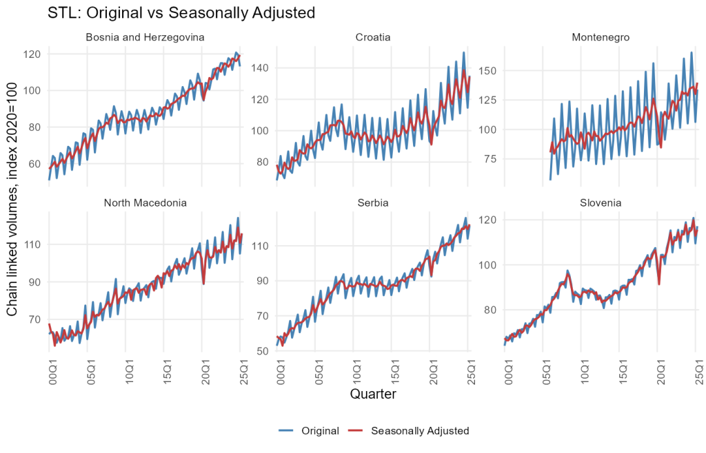
Bosnia and Herzegovina starts the period with the lowest index level but displays a remarkably steady upward trajectory. Growth is strong in the early 2000s, with a visible pause around the GFC, followed by renewed expansion. The pandemic shock appears as a sharp drop in 2020 followed by a relatively swift rebound, after which the level of real GDP continues to rise.

Croatia’s path is more uneven. From 2000 until the mid-2000s the trend is upward, but the GFC produces a deep and prolonged downturn. The seasonally adjusted series shows that Croatia’s output stagnated or declined for several years, not fully recovering its pre-crisis level until the mid-2010s. The pandemic then generates another sudden contraction, but the recovery is rapid and by the early 2020s real GDP is well above its pre-COVID level, consistent with stronger integration into EU value chains and, more recently, euro adoption.

Montenegro shows the most pronounced seasonal amplitude in the original series, reflecting the prominence of tourism and related services. The trend rises strongly over the sample, but with notable volatility: expansions are rapid, downturns are sharp, and the COVID-19 shock stands out as an exceptionally deep trough. Even in the seasonally adjusted series, the pandemic collapse dominates the picture, reminding us how exposed a small, tourism-dependent economy is to global travel disruptions.

North Macedonia and Serbia display somewhat smoother trajectories. Both exhibit solid trend growth in the early and mid-2000s, a visible slowdown during and after the GFC, and a relatively contained but still sharp decline in 2020. In the most recent years the seasonally adjusted series suggest steady, if not spectacular, gains in output. Slovenia, finally, begins the period at a higher index level, reflecting its earlier progress in transition and integration. Its trend increases strongly until the GFC, then experiences a sizeable and protracted downturn, more severe than in some neighbours, before a robust recovery sets in from around the mid-2010s onwards. The pandemic shock is clearly visible, but the subsequent rebound lifts the series to new highs by 2025.

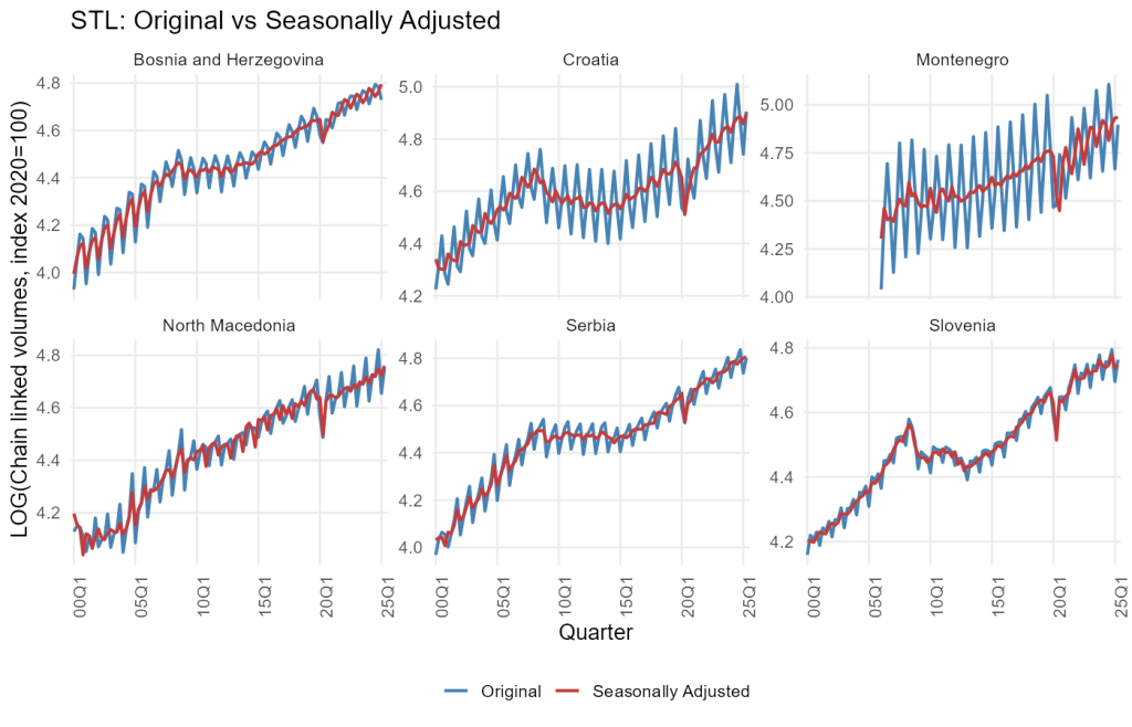
When the same analysis is repeated in logarithms, the log-transformed series look visually smoother in the upper part of the range (Figure 2). The log scale compresses large values and accentuates proportional rather than absolute changes, making it easier to compare growth rates across countries. Overall patterns, however, remain the same: a broad upward drift, a major interruption during the GFC, and a pronounced but temporary collapse during the pandemic.

2.2 Decomposition in levels and logs: trend, seasonality and irregular components

The STL decompositions for the level series in Figure 3 split each GDP index into three components: a slowly moving trend-cycle, a regular seasonal pattern, and an irregular remainder. In every country the trend-cycle component rises significantly over the quarter century, confirming that long-run growth is the dominant feature of these series. The upward sloping trend is particularly smooth for North Macedonia, Serbia and Slovenia, while Bosnia and Herzegovina, Croatia and Montenegro display somewhat more curvature, reflecting episodes of acceleration and deceleration.

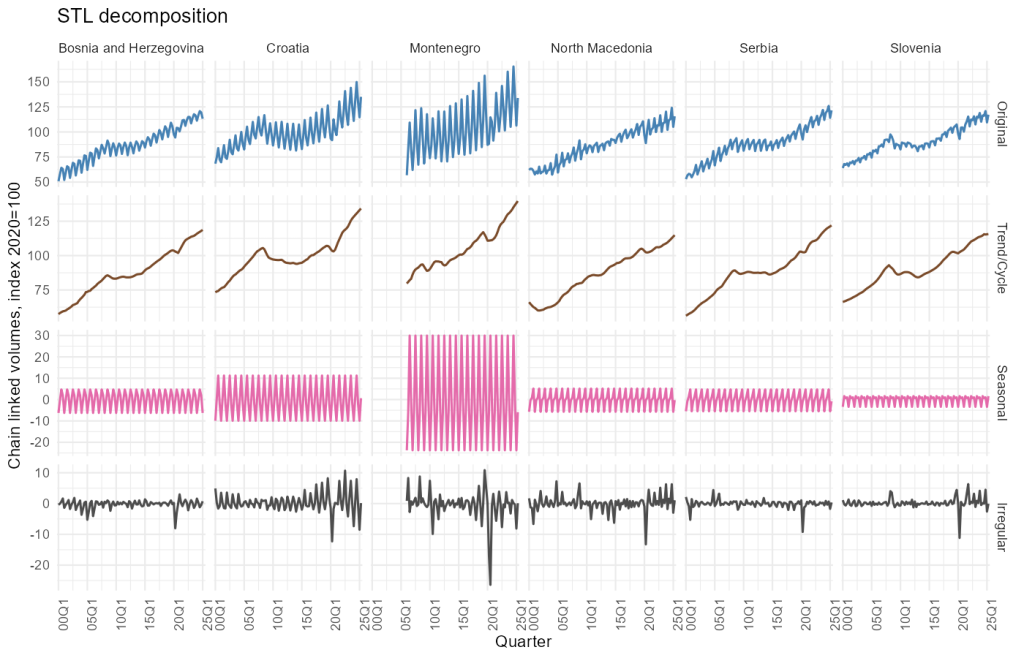
Seasonal components are strong across the region but differ in amplitude. Montenegro stands out with the largest seasonal swings, consistent with pronounced summer peaks and winter troughs driven by tourism. Bosnia and Herzegovina and Croatia also exhibit sizeable, regular seasonality, whereas Slovenia, North Macedonia and Serbia show more moderate seasonal variation. The seasonal pattern itself is highly stable over time in most countries, suggesting that the structure of the economy, and in particular the timing of activity within the year, has not drastically changed.

The irregular components capture shocks and noise that cannot be attributed to smooth trend or recurring seasonality. Here, the GFC and COVID-19 episodes are clearly visible as clusters of large residuals. In several countries, notably Croatia, Montenegro and Slovenia, the irregular component spikes during the late 2000s and early 2010s, indicating that the downturn associated with the GFC was not merely a gentle bending of the trend but involved abrupt shifts and volatility. The pandemic period shows even sharper irregular movements, especially in Montenegro and North Macedonia, where the 2020 collapse and subsequent rebound dominate the residual series.

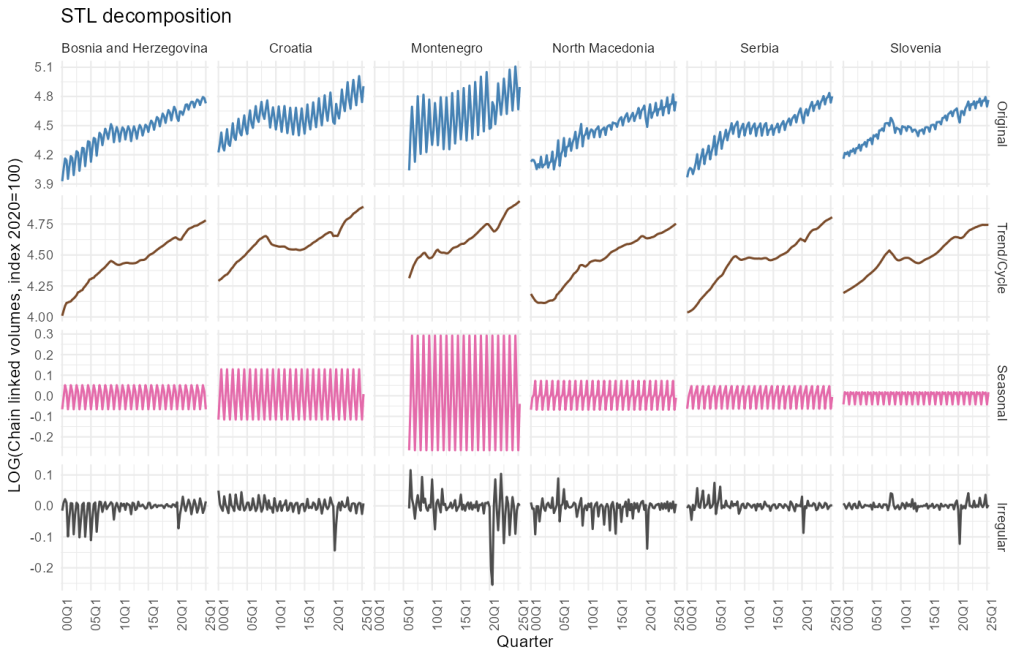
Repeating the decomposition on the log-transformed series yields similar insights but in proportional terms (Figure 4). The log-trend components show steady growth with slightly smoother slopes, while the seasonal components become roughly constant in amplitude, consistent with the idea that percentage seasonal effects have remained stable. The irregular components in logs highlight episodes where proportional changes were extreme, again emphasising the outsized impact of 2020.

2.3 Growth rates and differenced logs

Economists often think about GDP not only in levels but also in growth rates. Taking first and seasonal differences of the log series yields approximations to quarter-on-quarter and year-on-year growth rates. The corresponding graphs (Figure 5) show that once we difference the logs, most of the persistent trend disappears and the series fluctuate around zero.

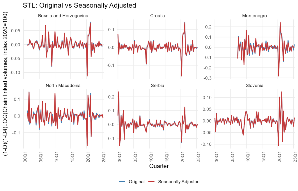
In this growth-rate view, the GFC appears as a sequence of negative observations and elevated volatility in the late 2000s and early 2010s, with Croatia and Slovenia again experiencing longer periods of weak or negative growth. The COVID-19 shock, however, is in a league of its own: every country shows an extraordinary negative spike in 2020, followed by unusually large positive values as activity rebounds. Montenegro’s spikes are the largest in magnitude, reflecting its heavy reliance on international tourism. Bosnian, Serbian and North Macedonian growth rates are also severely affected, but their rebounds appear somewhat more contained, perhaps because their sectoral mix is slightly more diversified.

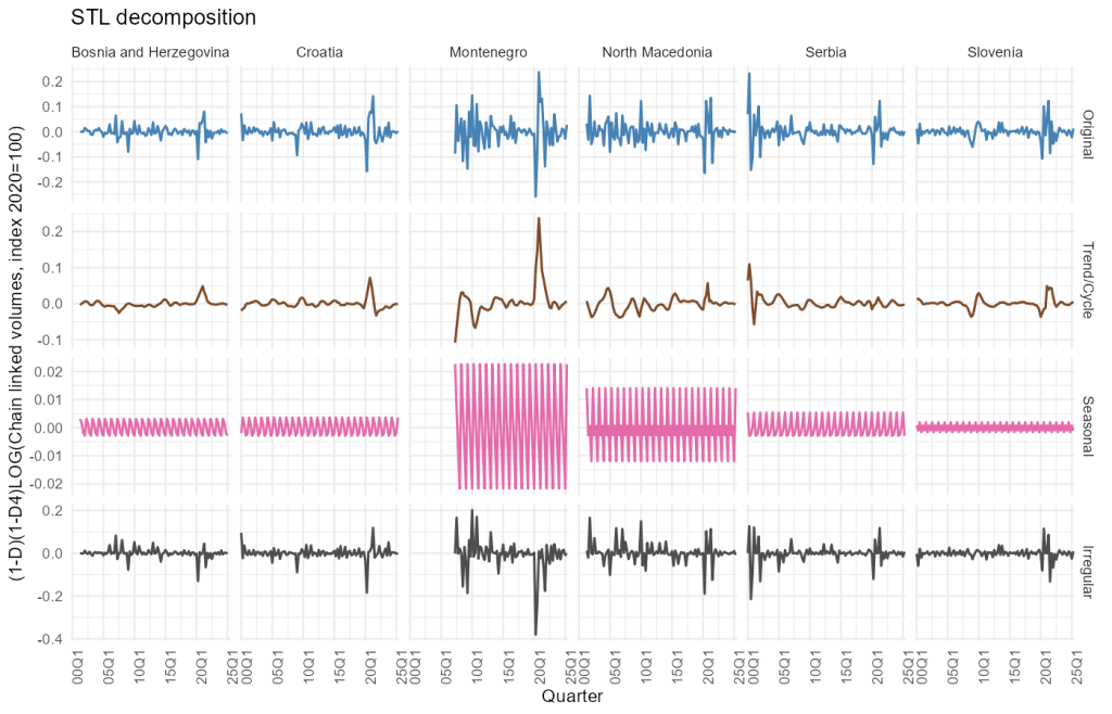
The STL decomposition of the differenced log series (Figure 6) confirms that, after differencing, seasonal effects are greatly reduced but not eliminated. A small residual seasonal pattern remains, particularly in countries with strong tourism or agricultural cycles. The trend-cycle component is now close to zero most of the time, with only gentle drifts, while the irregular component captures most of the action and again highlights the crisis periods. This decomposition underscores a familiar lesson: differencing is powerful in removing long-run drift but cannot, by itself, guarantee the absence of seasonality or irregular shocks.

2.4 Cross-country co-movement and the balance between trend and seasonality

The scatterplot matrices for the log series (Figure 7) reveal strong positive co-movement across the six economies. In levels and logs, pairwise correlations are high, often well above 0.7 and in some cases above 0.9, particularly between Slovenia and Serbia or between Slovenia and Bosnia and Herzegovina.

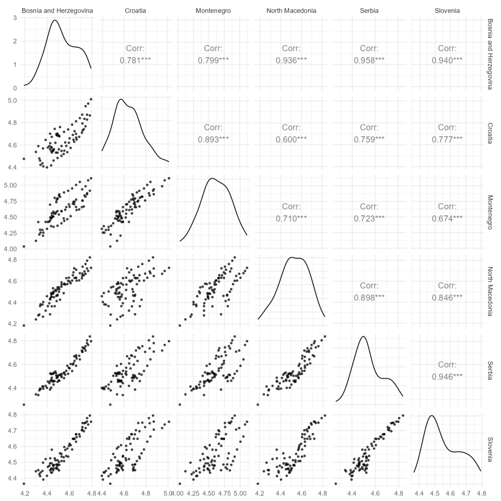
This degree of synchronicity is consistent with deep trade, financial and institutional integration with the European Union and with each other, as well as exposure to common external shocks such as the GFC and the pandemic.

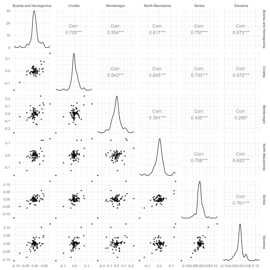
When we move to growth rates, correlations remain positive but become somewhat smaller and more dispersed (Figure 8). This is exactly what one would expect: long-run trends are influenced by common structural forces, convergence towards EU income levels, similar demographic dynamics and shared transition legacies, while short-term growth rates are also shaped by country-specific fiscal, monetary or structural policies, as well as idiosyncratic events.

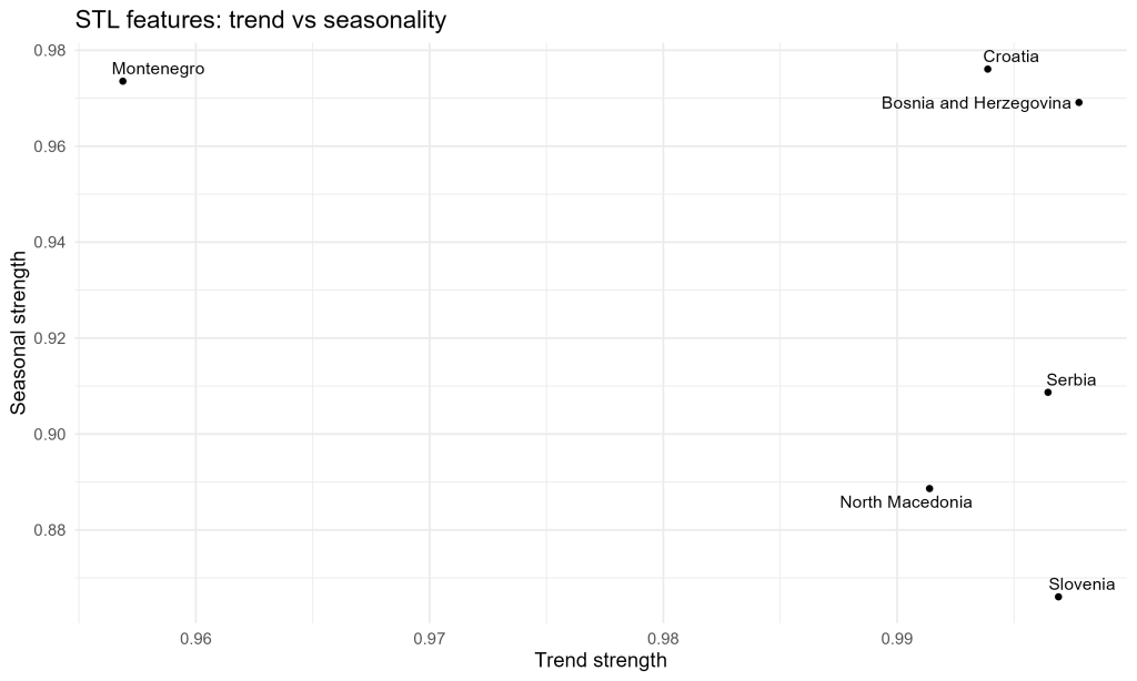
Figure 9 summarises the balance between trend and seasonality for the original series by plotting measures of trend strength against measures of seasonal strength derived from the STL decomposition. All countries sit in the upper-right portion of the diagram, indicating that both trend and seasonal components are very important. Yet there are meaningful differences. Slovenia, North Macedonia and Serbia exhibit exceptionally strong trend components combined with somewhat weaker seasonal components, implying that long-run growth and medium-term cycles account for most of the variation in their GDP indexes. Bosnia and Herzegovina and Croatia feature both strong trends and pronounced seasonalities, while Montenegro stands out with very strong seasonal strength relative to its trend, cementing its profile as the most seasonality-driven economy in the group.

3. Economic outlook

The most recent years of data, culminating in 2025Q2, suggest that all six economies have moved beyond the immediate fallout of the COVID-19 pandemic. Seasonally adjusted real GDP is at or above its pre-pandemic level everywhere, and the trend components indicate renewed expansion. However, the speed and robustness of this expansion differ across the region.

In Slovenia and Croatia the trend components show a decisive upward slope following the 2020 collapse, indicating that these EU and euro-area members have managed to leverage strong external demand, EU recovery funds and continued integration into global value chains. For Croatia, the tourism rebound is particularly visible in the renewed amplitude of seasonal peaks. Montenegro’s pattern is similar but more extreme. Its trend has recovered, but the irregular component remains volatile, and the seasonal pattern is as pronounced as ever. This underscores both the strength and vulnerability of a growth model heavily anchored in tourism: when the season is good, growth is strong; when it is disrupted, the economy suffers disproportionately.

Bosnia and Herzegovina and North Macedonia show steadier, if somewhat slower, post-pandemic growth. Their trend components slope upward, but without the dramatic acceleration visible in Croatia or Slovenia. For these economies, continued reforms and investment in infrastructure, human capital and institutions will likely determine whether they can sustain convergence towards EU income levels.

Serbia occupies an intermediate position. Its trend path indicates consistent growth over the sample, with relatively mild but clearly visible downturns during both the GFC and the pandemic. In the last few years the trend continues to rise steadily, while seasonality remains moderate compared with Montenegro or Croatia. From an economic-outlook perspective this suggests that Serbia has built a more diversified production base, less dependent on a single seasonal sector, but still subject to regional and global shocks through trade and financial channels.

Comparing the group to Serbia as a reference point helps clarify these nuances. Relative to Serbia, Slovenia and Croatia have experienced more pronounced cycles, with deeper downturns during the GFC but also stronger rebounds in the last decade, consistent with their earlier EU and euro-area integration. Montenegro displays much higher seasonal volatility and greater sensitivity to pandemic-related restrictions. Bosnia and Herzegovina and North Macedonia, in contrast, exhibit somewhat smoother trajectories, but their levels of real GDP remain lower and their convergence towards the EU average more gradual.

Looking ahead, the combination of strong trend components and persistent seasonality suggests that policy makers must manage both long-run structural issues and short-term seasonal vulnerabilities. In the more tourism-intensive economies, diversification and resilience to shocks affecting travel and services remain key. In the more industry- and services-diversified economies, the policy focus will be on sustaining investment, improving productivity and navigating external headwinds such as tighter global financial conditions, energy price volatility and geopolitical uncertainty.

4. Methodological appendix

4.1 Graphical exploration

The analysis begins with simple but powerful tools: time-series graphs. Plotting the original quarterly indices makes it possible to see at a glance whether a series is trending upward or downward, whether it exhibits seasonality, and where major breaks and turning points occur. Combining original and seasonally adjusted series on the same panels shows how much of the apparent short-run volatility is attributable to recurring intra-year patterns and how much reflects genuine changes in underlying activity.

Scatterplot matrices provide a complementary view by displaying pairwise relationships across countries. Diagonal density plots show the distribution of each series or transformation, while off-diagonal scatterplots reveal whether countries’ GDP movements are strongly synchronised or only loosely related. This combination of time-domain and cross-sectional plots is particularly useful in regional studies where common shocks and spillovers are important.

4.2 Transformations: logarithms and differencing

Real GDP indices measured as chain-linked volumes often show increasing variance as the level rises. Taking logarithms stabilises the relative variability, because proportional changes correspond to roughly constant differences in logs. In these graphs the log transformation compresses the upper part of the series and makes growth rates more comparable across countries.

Formally, if () denotes the GDP index in quarter (), the log-transformed series is defined as (). First differences () approximate quarter-on-quarter growth rates, while seasonal differences () approximate year-on-year growth for quarterly data. By plotting both the level series and their differenced logs we can simultaneously study long-run convergence and short-term fluctuations.

Differencing is also a practical step towards stationarity, an assumption underlying many time-series models. However, as the decompositions of the differenced log series show, differencing alone does not necessarily remove all seasonal structure, which is why dedicated seasonal adjustment procedures remain useful even after transformations.

4.3 Seasonal adjustment and decomposition using STL

Seasonal adjustment is the process of removing predictable intra-year patterns so that movements from one period to the next reflect underlying economic changes rather than the mechanical effects of seasons, holidays or institutional schedules. In this study the primary tool is STL, which decomposes the series into trend, seasonal and remainder components using locally weighted regressions (Loess).

In an additive decomposition the observed series is written as

where () denotes the trend-cycle, () the seasonal component, and () the irregular remainder. STL estimates these components iteratively. In each iteration, it smooths the series across seasons to estimate (), smooths seasonally adjusted residuals across time to estimate (), and assigns whatever is left to (). Loess smoothing windows and robustness weights control how quickly the trend and seasonal components can change and how much influence outliers have.

STL has several advantages that are particularly relevant for this dataset. It can handle long series with complex seasonal patterns, allows the strength of seasonality to evolve gradually over time, and is robust to extreme values such as those observed during the pandemic. Moreover, because it is non-parametric, it avoids the need to specify a particular ARIMA model for each country, which would be cumbersome in a multi-country comparison.

4.4 Alternative seasonal adjustment methods: X-13ARIMA-SEATS and TRAMO/SEATS

While STL is flexible and transparent, many official statistics agencies rely on model-based seasonal adjustment procedures. The most widely used is X-13ARIMA-SEATS, developed by the U.S. Census Bureau. X-13 combines two elements. The first is an ARIMA modelling step that handles calendar effects, outliers and short-term dynamics. The second is a decomposition step using either the traditional X-11 filter-based method or the SEATS model-based signal extraction technique, which derives the trend, seasonal and irregular components from the estimated ARIMA model. X-13 offers extensive diagnostics and is the de facto standard in many national statistical offices, but it requires more modelling choices and expertise than STL.

Another prominent option is TRAMO/SEATS, developed at the Banco de España. TRAMO (Time Series Regression with ARIMA Noise, Missing Observations, and Outliers) pre-adjusts the series by fitting a regression-ARIMA model that can accommodate missing data and various types of outliers. SEATS (Signal Extraction in ARIMA Time Series) then decomposes the fitted model into unobserved components corresponding to trend, seasonal and irregular movements. TRAMO/SEATS is strongly grounded in econometric theory and often delivers smooth and economically interpretable trend-cycles. It is officially recommended or used by several European and international organisations.

Compared with these model-based methods, STL’s main strengths are its flexibility, robustness and ease of use in exploratory work. It is particularly attractive when the analyst needs to process many series consistently or wishes to avoid the complexities of ARIMA specification. Model-based methods such as X-13ARIMA-SEATS and TRAMO/SEATS, by contrast, may provide better long-run extrapolation, richer diagnostics and a clearer link between statistical assumptions and economic interpretation, at the cost of greater complexity and sensitivity to model mis-specification. In practice, many statistical agencies use model-based procedures for official figures while STL and related approaches play a complementary role in research and exploratory analysis.

5. Conclusion

The quarterly real GDP indices for Bosnia and Herzegovina, Croatia, Montenegro, North Macedonia, Serbia and Slovenia from 2000 to 2025 tell a story of long-run growth interrupted by two major crises. The STL decompositions show that trend components rise substantially in all six countries, confirming that, despite setbacks, the region has moved to a much higher level of output. Seasonal patterns, though strong, are highly regular and in most cases stable, with Montenegro, Bosnia and Herzegovina and Croatia displaying the most pronounced seasonal swings. Irregular components highlight the severity of the GFC and, even more so, the COVID-19 shock.

Scatterplot matrices and feature plots indicate a high degree of co-movement across the region, especially in levels and logs, reflecting shared exposure to European and global shocks and deepening economic integration. Differences emerge more clearly in growth rates and in the balance between trend and seasonal strength. Montenegro’s GDP is the most seasonality-driven; Slovenia and North Macedonia have the strongest trend components; Croatia and Bosnia and Herzegovina sit between these poles; and Serbia occupies a relatively balanced position, with a robust trend and moderate seasonality.

Using Serbia as a reference point, we can say that its growth path has been relatively smooth, with less dramatic boom-bust cycles than in some neighbours, but also without the exceptionally strong post-GFC rebound seen in Slovenia. Croatia’s and Montenegro’s greater seasonality exposes them to larger short-term swings, especially in crises that hit tourism hard. Bosnia and Herzegovina and North Macedonia continue to grow but at a more measured pace, underscoring the importance of structural reforms to accelerate convergence.

Beyond their immediate descriptive value, these results illustrate the broader usefulness of combining transformations, seasonal adjustment and graphical analysis in macroeconomic work. By looking at levels, logs and growth rates, and by decomposing each series into trend, seasonal and irregular components, we obtain a nuanced picture of how economies evolve through time, how they respond to shocks, and how they resemble or differ from one another. The same toolkit can be readily applied to other macroeconomic indicators, industrial production, wages, prices or tourism, providing a consistent framework for tracking the economic pulse of the former Yugoslav region in the years to come.

References

Cleveland, R. B., Cleveland, W. S., McRae, J. E., & Terpenning, I. (1990). STL: A seasonal-trend decomposition procedure based on Loess. Journal of Official Statistics, 6(1), 3–73. https://www.math.unm.edu/~lil/Stat581/STL.pdf

Eurostat. (2025a). National accounts and GDP – Statistics explained. European Commission. https://ec.europa.eu/eurostat/statistics-explained/index.php/National_accounts_and_GDP

Eurostat. (2025b). Gross domestic product (GDP) and main components (output, expenditure and income), quarterly – Chain linked volumes, index 2020 = 100 (namq_10_gdp). Retrieved from Eurostat database.

Gómez, V., & Maravall, A. (1996). Programs TRAMO and SEATS: Instructions for the user. Banco de España. https://www.bde.es/f/webbde/SES/Secciones/Publicaciones/PublicacionesSeriadas/DocumentosTrabajo/96/Fich/dt9628e.pdf

U.S. Census Bureau. (2025). X-13ARIMA-SEATS seasonal adjustment program: Reference manual. U.S. Department of Commerce. https://www.census.gov/data/software/x13as.html

Hyndman, R. J. (2025). Forecasting: Principles and practice (3rd ed.). OTexts. https://otexts.com/fpp3