This post analyses in two parts Serbia’s quarterly Construction index (base 2021 = 100) over 2000Q1–2024Q4. The tone is deliberately “macro-for-educated-readers”, but the logic is firmly time-series: separate the long-run trajectory from regular seasonal swings, then ask what remains, and whether that “remainder” lines up with the broader GDP cycle.

Part 1 — Levels, seasonal adjustment, and decomposition

1. Introduction

Construction is one of those sectors that rarely moves quietly. It is capital-intensive, politically salient, and unusually exposed to timing frictions: procurement cycles, weather constraints, financing conditions, and the stop–go rhythm of infrastructure projects all leave fingerprints in the data. In macro terms, construction is both a mirror (reflecting demand, credit, and confidence) and a lever (public investment and housing booms can move the aggregate cycle).

The data here cover a long span, 2000Q1 to 2024Q4, and what immediately stands out is that Serbia’s construction series is not just trending upward; it is doing so while carrying a large, regular seasonal pulse that repeats year after year. That combination is analytically tricky: the raw series can look volatile even when the underlying direction is stable, and the underlying direction can look stable even when turning points are forming underneath the seasonal noise. That is why the first half of the analysis focuses on seasonal adjustment and decomposition, using two standard approaches, STL and X-13ARIMA-SEATS, to make the same story readable in two different “statistical dialects.”

2. What the raw series hides, and what adjustment reveals

Figures 1 and 2 plot the original series against seasonally adjusted versions. The raw quarterly path shows a repeated within-year pattern: low quarters are followed by catch-up quarters, followed by peaks, and then another reset. That pattern is not a minor decorative feature; it is large enough that, without adjustment, you would routinely mistake seasonal rebounds for structural acceleration, and seasonal slowdowns for macro weakness.

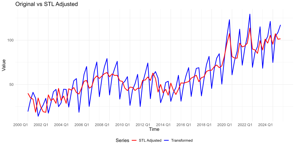
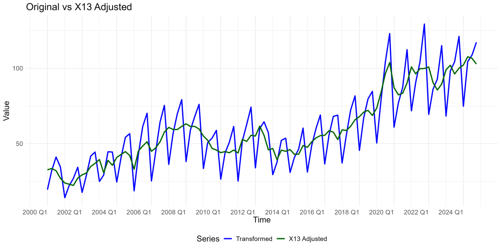
Once seasonality is removed, the adjusted series makes the medium-run narrative clearer. First, the 2000s look like a long climb, culminating in a late-2000s high. Second, there is a visible weakening and flattening in the early 2010s. Third, from the mid-to-late 2010s onward the series resumes a firmer rise, and in the early 2020s it sits on a distinctly higher plateau than in the prior decade. (The visual jump in the early 2020s is large enough that it reads like a regime change rather than “just another good year.”)

An important practical point is that the two adjustment methods, STL (Figure 1) and X-13 (Figure 2), tell broadly the same story. That agreement matters: when two different methods produce similar adjusted paths, you gain confidence that the “headline narrative” is not a fragile artefact of one particular procedure.

3. Decomposition: trend, seasonality, and the irregular

Figures 3 and 4 decompose the series into components. The STL decomposition (Figure 3) presents the observed series as an additive sum of trend, seasonal, and irregular parts; the X-13 decomposition (Figure 4) is presented in a way that typically corresponds to a multiplicative interpretation (seasonal and irregular components shown as factors around 1). Those are different representations, but they are answering the same macro question: what is persistent, what is calendar-regular, and what is genuinely “surprising”?

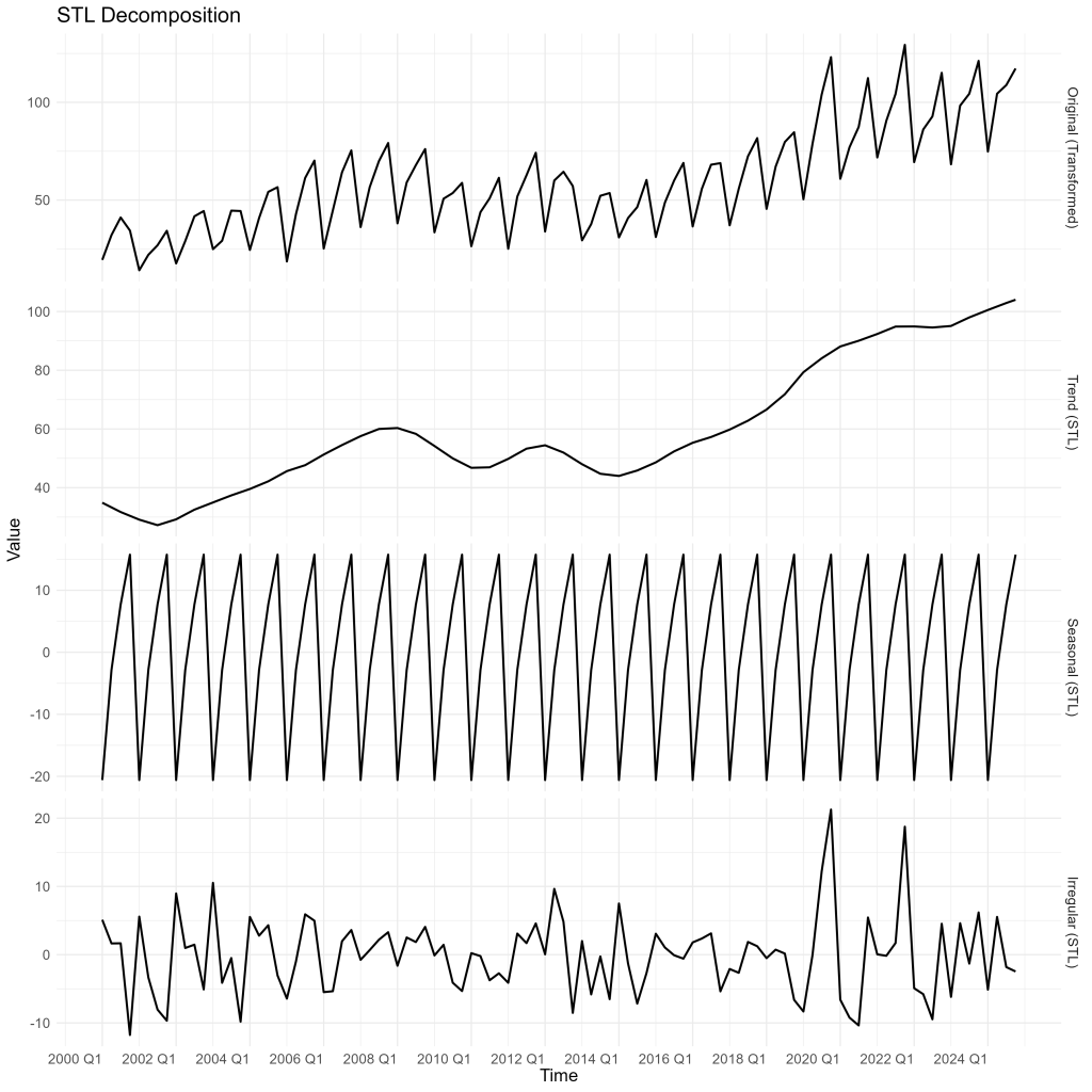
The trend component is the backbone. In STL, it rises through the 2000s, rolls over around the global financial crisis window, and then re-accelerates in the second half of the sample, with especially strong momentum into the early 2020s. In X-13, the trend tells the same story but with slightly different curvature: the late-2010s rise is more visibly step-like, and the early-2020s segment looks like a move to a higher level followed by consolidation.

The seasonal component is the metronome. In STL it is strikingly stable: the within-year “shape” repeats with similar amplitude year after year, which is exactly what you would expect when weather and work scheduling dominate the quarter-to-quarter timing. In X-13 the seasonal factor similarly oscillates with a regular quarterly rhythm around 1. The key macro implication is that Serbia’s construction activity does not merely have seasonality; it has strong and durable seasonality, meaning you should almost never interpret a single-quarter change in the raw series at face value.

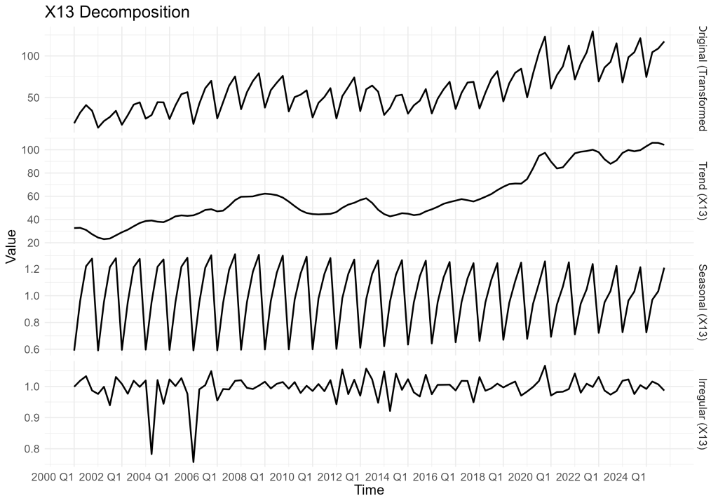
The irregular component is where shocks, outliers, and measurement quirks live. In STL, the irregular swings are usually modest but punctuated by a handful of large spikes; in X-13, the irregular factor mostly hugs 1 with several noticeable deviations. This is where the analyst’s discipline matters: you can hypothesise about events, but you should only do so when the timing and magnitude are visually compelling. Here, two windows stand out as visually “non-routine”: a downturn around the late-2000s/early-2010s and unusual volatility around the early 2020s. Those are the only periods that plausibly justify event-language such as “GFC-era weakness” or “pandemic-era disturbance,” because those are the periods where the component plots visibly depart from their usual behaviour.

4. STL vs X-13 in practice: adjusted series and trends

Figures 5 and 6 put the two methods side by side. Figure 5 compares the seasonally adjusted series. The takeaway is not rivalry but robustness: the two lines largely track each other, meaning the big macro features, rise, flattening, re-acceleration, high early-2020s level, are not sensitive to the method.

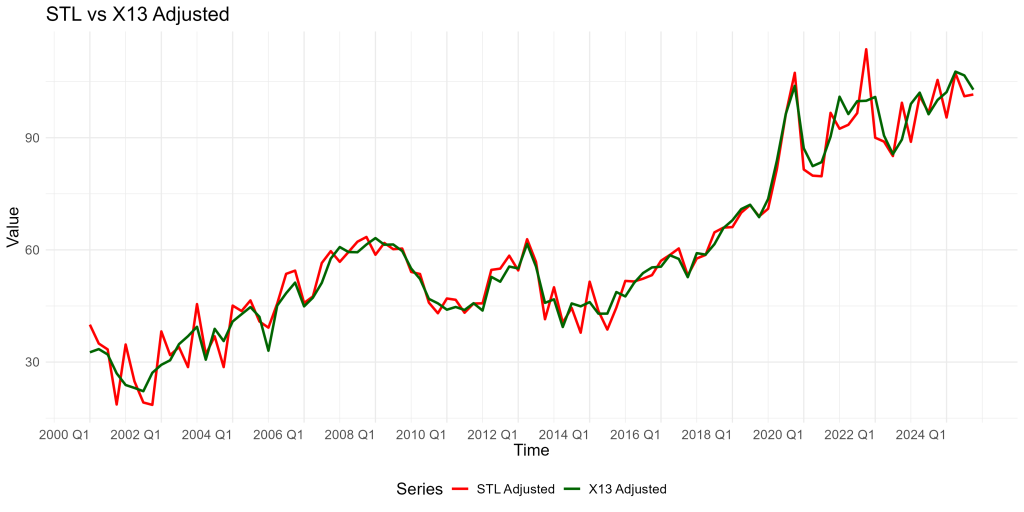
Where they differ is in the “texture.” STL, built on local smoothing, tends to produce an adjusted series that can be a bit more responsive to short-run movements. X-13, built on a model-based structure, can sometimes look slightly more conservative in how it allocates movements between trend-cycle and irregular components. That difference becomes more visible when the underlying series contains abrupt shifts or unusually large quarter-specific movements.

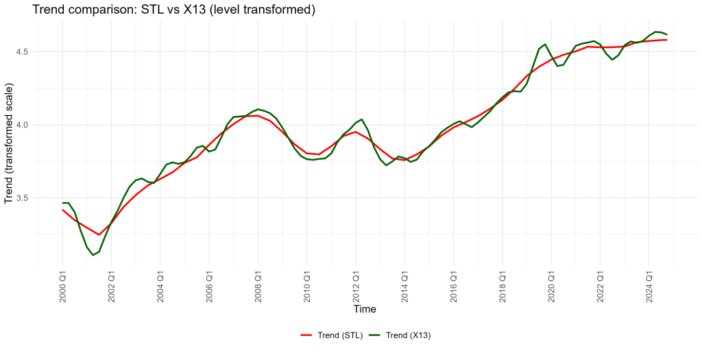
Figure 6 compares trends on a transformed (log) scale. The two trend lines are again close, but X-13 appears somewhat more “wiggly” in certain stretches, while STL is smoother. A good way to read this is: both agree on the direction and major turning points, but they disagree slightly on how quickly the economy moved between those states. For macro interpretation, the shared message is far more important than the stylistic differences.

5. Seasonal diagnostics: what the year looks like in construction

Figures 7–9 zoom in on seasonality.

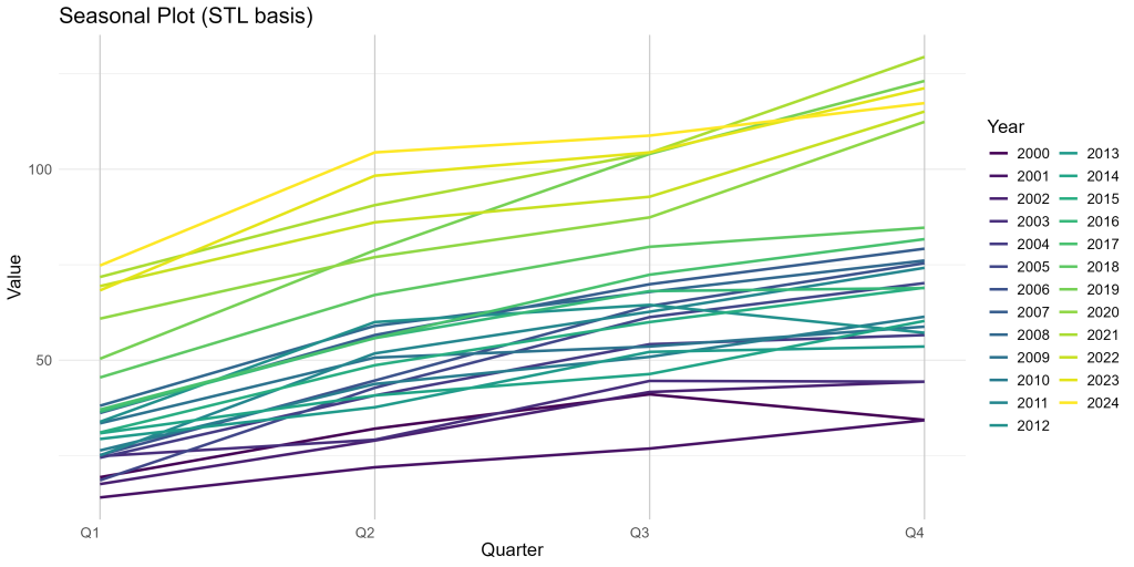
Figure 7 (seasonal plot) shows a remarkably consistent within-year profile: construction is typically weakest early in the year and strengthens as the year progresses, with the highest levels appearing late in the year. The slope from Q1 to Q4 is visible for most years, suggesting a structural calendar mechanism rather than a one-off phenomenon.

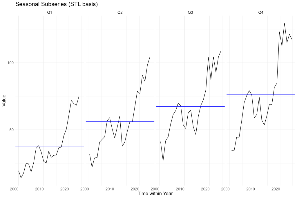
Figure 8 (seasonal subseries) makes the quarter-by-quarter pattern even clearer. Each quarter has its own “band,” and the mean level differs systematically across quarters. The within-quarter histories also show that the post-2020 period is not simply “the same seasonal pattern at a higher level”; it is also a period where some quarters (especially later quarters) appear to occupy a distinctly higher range than before, consistent with a higher-activity regime.

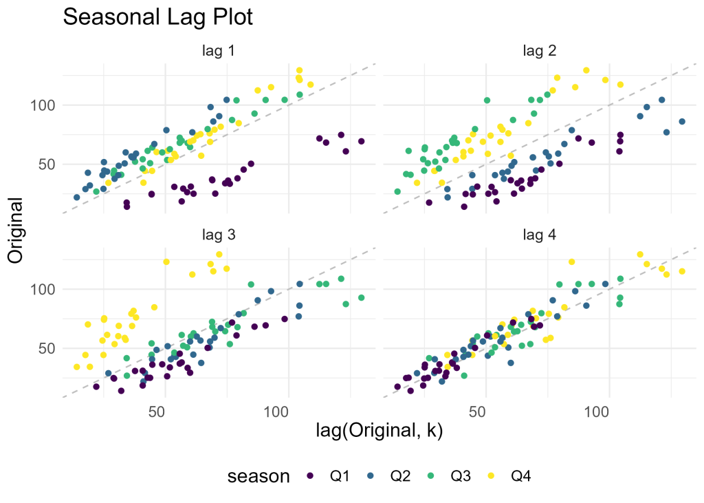
Figure 9 (seasonal lag plot) is a compact way of seeing persistence. The strongest alignment appears at the seasonal lag (effectively “this quarter vs the same quarter last year”), which is exactly what you would expect in a quarterly series with stable seasonality. The clustering by quarter colour reinforces the story: the series has memory, and it has seasonal memory.

6. Conclusion (Part 1)

The first half of the evidence is straightforward but economically meaningful. Serbia’s construction series over 2000–2024 is best described as trend-driven growth plus strong seasonality, with a visible soft patch around the late-2000s/early-2010s and a markedly higher level in the early 2020s. The most reassuring methodological point is that two different seasonal adjustment systems, STL and X-13, converge on the same macro narrative.

If you only remember one lesson from Part 1, it should be this: in a series with seasonality this strong, the raw quarterly path is not “noise”, it is systematic calendar structure. The correct macro question is therefore never “what happened this quarter?” but “what happened to the seasonally adjusted trend and cycle?”

7. Methodological appendix (Part 1): STL and X-13, and why transforms matter

The workflow in Part 1 is deliberately graphical because time-series failures often begin as visual misreadings: confusing seasonal rebounds for growth, mistaking a one-off shock for a turning point, or ignoring that volatility tends to scale with the level of activity. When variance rises as the series rises, analysts often apply a log transform (or a Box–Cox transform) to stabilise fluctuations and make proportional changes comparable over time.

STL (Seasonal-Trend decomposition using Loess) treats the observed series as the sum of a trend, a seasonal pattern, and an irregular remainder. It estimates these pieces by iterative local smoothing, which makes it flexible and robust, especially useful when seasonality is stable but the trend evolves gradually. X-13ARIMA-SEATS is model-based: it uses regression and ARIMA modelling to pre-adjust the series and then applies signal extraction to split the movement into trend-cycle, seasonal, and irregular components. In practice, the strength of X-13 is standardisation and diagnostics; the strength of STL is transparency and adaptability. When both are applied to the same series, as here, the best outcome is not that one “wins,” but that they broadly agree, because that suggests the economic story is not an artefact of one particular statistical lens.

References (Part 1)

Cleveland, R. B., Cleveland, W. S., McRae, J. E., & Terpenning, I. (1990). STL: A seasonal-trend decomposition procedure based on Loess. Journal of Official Statistics, 6(1), 3–73.
Findley, D. F., Monsell, B. C., Bell, W. R., Otto, M. C., & Chen, B.-C. (1998). New capabilities and methods of the X-12-ARIMA seasonal-adjustment program. Journal of Business & Economic Statistics, 16(2), 127–152.
U.S. Census Bureau. (n.d.). X-13ARIMA-SEATS seasonal adjustment program.