Before the tests, the charts already tell a story, just not a tidy one.

The full econometric methodology behind this Serbia exercise was explained in a separate blog post. This instalment stays deliberately visual and intuitive: what the data seem to say before we ask them to pass any formal statistical exams.

1. Why Serbia makes Okun’s Law squirm

Okun’s Law is often treated as the macroeconomist’s pocket translator: if output rises faster, unemployment should drift down; if output stalls, joblessness should rise. Serbia does not reject that translation outright. It simply insists on speaking with an accent, sometimes thick, sometimes barely audible.

The study’s first and most useful move is to separate two stories that get conflated in everyday commentary. One is the long-run trajectory: output rising over decades, unemployment (eventually) trending down. The other is the short-run cycle: abrupt contractions, partial recoveries, and the labour market’s stubborn tendency to adjust late and unevenly.

As shown in Figure 1 in Serbia’s case, the long-run picture is uncontroversial: log real GDP per capita generally rises over 1995–2024, but with visible disruptions in the early 2000s, during the global financial crisis, and again in 2020. The unemployment rate’s path is less smooth: elevated early on, some improvement mid-2000s, deterioration after 2008, and a pronounced decline from 2014 onward. That combination, the economy recovering on a trend while the labour market improves in lumps, already hints at the core theme of this post: in Serbia, output and unemployment co-move most clearly when something breaks, not when things merely improve.

2. Two Okuns in plain English: Changes and gaps

The study frames the relationship in two ways, both intuitive. The “first-difference” view looks at growth and changes in unemployment, good for capturing year-to-year movement and crisis spikes. The “gap” view tries to measure slack: how far output is from its trend (potential) and how far unemployment is from its trend (a natural rate), then asks whether those two deviations move in opposite directions.

Each approach comes with a trade-off that matters for policy interpretation. First differences are closer to the headlines, growth this year, unemployment change this year, but they are noisy and often contaminated by lags, composition shifts, and one-off events. Gaps aim to be more structural, capturing whether the economy is running hot or cold, but they depend on how you estimate the trend, and therefore can be “right” in a way that still feels fragile.

In this Serbia study, the gap concept is implemented through the Hodrick–Prescott filter. The point is not to fetishise the filter; it is to obtain a consistent way to talk about “above-trend” and “below-trend” periods without pretending that a single year’s growth rate tells the whole story.

3. The time-series story: output, unemployment, and the rhythm of adjustment

When you shift from levels to year-to-year changes, the Okun intuition becomes easier to see, and easier to misunderstand.

In the first-difference plot (Figure 2), GDP growth is “visibly more volatile” than the level series, with major contractions in 1999, 2009, and 2020, events the study explicitly links to the Kosovo conflict, the global financial crisis, and COVID-19. In each downturn, unemployment faces upward pressure, which fits the Okun narrative. And in several years of strong growth, such as 2004 and 2016–2018, unemployment tends to decline.

But the study refuses to let the reader conclude “growth mechanically fixes jobs.” It underlines that there are years where output growth coincides with stagnant or rising unemployment, plausibly reflecting labour-market adjustment lags or demographic influences. In other words: the sign is often right, the timing often isn’t, and the magnitude is not stable enough to be used as a single-rule policy autopilot.

4. Slack made visible: Output gap vs unemployment gap

If the first-difference view is the news cycle, the gap view is the business cycle.

The study’s HP-filter output gap is defined as the difference between actual GDP and the trend component of the filter (the estimated potential output). As shown in Figure 3 the output gap turns negative in underperformance periods and positive in above-trend periods, with major negative gaps around 2000–2002, 2009–2011, and 2020–2021, and shorter positive gaps around 2005–2007 and 2017–2019.

That matters because it provides a more narrative-friendly definition of recessions and recoveries: not simply “growth slowed,” but “the economy fell below its own trend,” which is closer to the language of stabilisation policy. The study explicitly presents the output gap as “a more stable measure of economic slack than simple annual growth,” precisely to set up a cleaner Okun story: unemployment should respond to cyclical deviations from potential, not merely to the latest growth print.

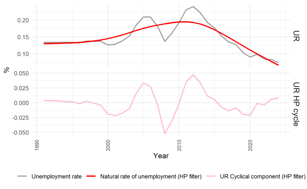
The unemployment-gap graph complements this (Figure 4). The study defines the unemployment gap as the deviation of actual unemployment from its HP-filtered “natural” rate, and it finds positive unemployment gaps (excess labour supply) in the same downturn windows that produce negative output gaps. 2001–2003, 2009–2012, and 2020, while recoveries such as 2006–2008 and 2017–2019 narrow the gap or push it negative (tighter labour market conditions). The study also notes a subtle but policy-relevant asymmetry: the unemployment gap often shows more inertia than the output gap, suggesting slower labour-market adjustment; and even in high-growth years Serbia “rarely experiences large negative unemployment gaps,” hinting at persistent structural issues or mismatch that keep slack from fully disappearing.

Those details matter because they tell you what Okun’s Law is for. It is not a prophecy that unemployment will fall whenever GDP rises. It is a way of thinking about cyclical slack and labour-market adjustment speed, how quickly the jobs side of the economy acknowledges what the output side is doing.

5. Regression-by-eye: What the scatter suggests (and what it doesn’t)

Now comes the part where many readers expect a clean payoff: the scatterplot should show a tidy downward slope, the regression line should confirm it, and the Okun coefficient should emerge like a well-behaved character in a nineteenth-century novel.

Serbia does not oblige.

The study constructs scatterplots for both the first-difference model and the gap model, including both “standard” direction (output predicting unemployment changes) and a reverse-causality framing. In the first-difference scatterplots, the study says the slope is “mildly negative” in the standard direction, consistent with Okun’s Law, but “not statistically significant,” with considerable dispersion; and the reverse direction is also weak and unstable.

But per your selective-figure rule, we will anchor the visuals here on the gap model, while still commenting on both.

In the gap scatterplots, the study again finds negative relationships in both directions, output gap versus unemployment gap (Figure 5) and its reverse (Figure 6), but describes them as “weak and statistically insignificant,” with data dispersion that looks much like the first-difference model’s noise. The study explicitly cautions that the gap specification does not automatically “capture underlying economic dynamics more reliably than simple differencing” in this Serbia sample, because the fit and outlier sensitivity remain similar.

That result is more meaningful than it sounds. It is not a failure of Okun’s intuition. It is a warning about what we can demand from a short annual sample in an economy with large shocks. The “Okun channel” can be real while still being hard to estimate precisely in a scatterplot regression, because the scatterplot is trying to compress a complex adjustment process (lags, sectoral shifts, participation, crisis distortions) into one line.

6. When one year breaks the model: Simple regressions, dummies, and the limits of patchwork

The study does not stop at scatterplots; it runs simple linear regressions for both Okun formulations and then asks the obvious question: what happens if an extraordinary year is not just another dot, but a rupture?

It introduces a dummy for 1999, explicitly tied to the Kosovo conflict and NATO bombing, to test whether “extreme conditions” distort the GDP–unemployment relationship and whether Okun’s Law survives that kind of stress test. The logic is intuitive: if your sample contains a year where output collapses for reasons that are not “the business cycle,” then a simple cyclical relationship can look artificially weak or unstable.

Yet the study’s message is again sober. In the piecewise/dummy-augmented regression, the 1999 dummy enters with the expected sign but is statistically insignificant; model fit improves only marginally; and the unemployment-gap segment coefficients remain unstable and weak. The interpretation is almost a policy lesson in itself: dummies can isolate one-off shocks, but they rarely restore a clean structural relationship when the underlying economy has experienced deeper discontinuities.

The study also draws a practical modelling conclusion that is very much within the graphical-analysis boundary: treating the unemployment gap as the dependent variable tends to produce “the most stable and interpretable result,” whereas modelling the output gap as dependent is more sensitive to episodes and yields coefficients that look unstable across periods. In plain English: unemployment appears to respond to output fluctuations more regularly than output responds to unemployment slack, at least in this descriptive-and-simple-regression stage.

The policy implication is sharpened further. The study argues that unemployment gaps can be “trusted as cyclical indicators” in Serbia, while output gaps are “more vulnerable to distortions from structural change and crises.” It advises policymakers to rely more on labour-market-based measures of slack and treat output-gap estimates with greater caution, particularly around crisis or transition episodes.

This is a subtle but important point for an informed general reader. In practice, governments and central banks often talk as if the output gap is the master variable, once you have it, everything else follows. The study is suggesting the reverse hierarchy may be safer in Serbia: treat labour-market slack as the sturdier indicator, and regard output-gap measures as more fragile, especially when history has not been kind to smooth trends.

7. What Part I can conclude, and what it must not

So where does this leave Okun’s Law in Serbia, at least at the “charts and simple regressions” stage?

It leaves it alive, but conditional.

The co-movement is clearest in crisis years: output contractions coincide with upward pressure on unemployment, and recoveries tend to coincide with declines in unemployment, though not with clockwork precision. The gap framework provides an intuitively appealing way to see slack and its labour-market counterpart, and the output and unemployment gaps often show a symmetry that supports the gap version conceptually, even while the scatter/regression fit remains weak and noisy.

But Part I also makes clear what we cannot honestly claim from pictures alone: that Serbia has a stable, precisely measurable Okun coefficient that can be used as a reliable policy rule year after year. The simple regressions and scatterplots are statistically weak; outliers matter; and extraordinary episodes do not submit politely to one-period dummies.

That is not an econometric nuisance. It is the substantive story: Serbia’s macro history creates conditions under which the Okun relationship can be present, but hard to pin down without tools designed for instability.

8. Bridge to Part II: The formal tests Serbia’s data will have to pass

Part II moves from “what the charts suggest” to “what the data will support when interrogated properly.” The study itself foreshadows why that matters: the instability hinted at in the visual stage, crisis disruptions, regime-like shifts, and weak simple-regression fit, creates a strong case for formal testing that can handle fragile time-series behaviour and structural episodes, before drawing any hard conclusions about long-run relationships or direction of influence.

In other words: if Okun’s Law is going to be trusted in Serbia, it must earn that trust the hard way.