
ARIMA Estimation and Short-Term Forecasting
2.1 From time-series structure to forecasting
Part 1 showed that Serbia’s GDP has strong trend, persistence and seasonality. Part 2 asks whether this structure can be captured well enough to produce useful short-term forecasts. The forecasting model used here is an ARIMA model estimated on the log-transformed GDP series. ARIMA models do not explain GDP using separate macroeconomic drivers such as consumption, investment, exports or fiscal policy. Instead, they forecast the future from the statistical structure of the series itself: its persistence, its past shocks and its seasonal behaviour.
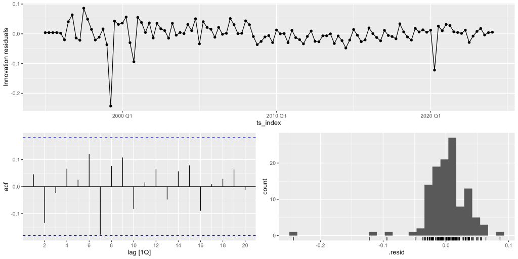
Table 2 reports an ARIMA specification with a strong autoregressive component, a moving-average term, a seasonal moving-average term and a constant. The autoregressive coefficient is about 0.916 and is estimated very precisely. This confirms the persistence already visible in the autocorrelation function. Economically, it means that shocks to the GDP path do not disappear immediately. A high or low movement in one quarter tends to influence subsequent quarters, although the effect gradually fades.
Table 2. ARIMA model estimation and parameters accuracy
| Model | arima | ets | naive | snaive |
|---|---|---|---|---|
| sigma2 | 0.001 | 0.001 | 0.007 | 0.003 |
| log_lik | 210.130 | 108.428 | NA | NA |
| AIC | -410.260 | -198.856 | NA | NA |
| AICc | -409.699 | -197.174 | NA | NA |
| BIC | -396.623 | -173.997 | NA | NA |
| MSE | NA | 0.001 | NA | NA |
| AMSE | NA | 0.002 | NA | NA |
| MAE.x | NA | 0.024 | NA | NA |
| lb_stat | 9.689 | 12.143 | 209.048 | 49.737 |
| lb_pvalue | 0.085 | 0.033 | 0.000 | 0.000 |
| .type | Test | Test | Test | Test |
| ME | -0.001 | -0.003 | 0.082 | 0.044 |
| RMSE | 0.008 | 0.011 | 0.090 | 0.046 |
| MAE.y | 0.007 | 0.010 | 0.082 | 0.044 |
| MPE | -0.012 | -0.065 | 1.708 | 0.923 |
| MAPE | 0.144 | 0.203 | 1.708 | 0.923 |
| MASE | NA | NA | NA | NA |
| RMSSE | NA | NA | NA | NA |
| ACF1 | -0.213 | 0.088 | -0.288 | 0.173 |
| estimate__ar1 | 0.916 | NA | NA | NA |
| std.error__ar1 | 0.053 | NA | NA | NA |
| statistic__ar1 | 17.303 | NA | NA | NA |
| p.value__ar1 | 0.000 | NA | NA | NA |
| estimate__ma1 | -0.284 | NA | NA | NA |
| std.error__ma1 | 0.130 | NA | NA | NA |
| statistic__ma1 | -2.190 | NA | NA | NA |
| p.value__ma1 | 0.031 | NA | NA | NA |
| estimate__sma1 | -0.817 | NA | NA | NA |
| std.error__sma1 | 0.074 | NA | NA | NA |
| statistic__sma1 | -11.050 | NA | NA | NA |
| p.value__sma1 | 0.000 | NA | NA | NA |
| estimate__constant | 0.003 | NA | NA | NA |
| std.error__constant | 0.000 | NA | NA | NA |
| statistic__constant | 5.093 | NA | NA | NA |
| p.value__constant | 0.000 | NA | NA | NA |
The moving-average coefficient is negative and statistically significant. This suggests that short-run innovations are partly corrected in subsequent quarters. The seasonal moving-average coefficient is also strongly negative and highly significant, which is consistent with the strong quarterly seasonal structure identified in Part 1. The constant term is positive and statistically significant, reflecting the underlying growth tendency in the transformed series.
The residual diagnostics are broadly acceptable. The Ljung-Box p-value for the ARIMA model is around 0.084. At the conventional 5% level, this means that the null hypothesis of no remaining residual autocorrelation is not rejected. The result is not so large that the model can be treated as flawless, but it is good enough for a practical short-term forecasting model. Figure 4 tells the same story visually. Most residuals fluctuate around zero, but there is a very large negative residual around 1999 and another visible disturbance around 2020. These are not ordinary forecasting errors; they correspond to exceptional historical shocks that a univariate model cannot be expected to anticipate fully.
Table 2 also compares the ARIMA model with simpler benchmarks. On the holdout sample, the ARIMA model has a much lower MAPE than the naive and seasonal naive alternatives and also performs better than the ETS model. This matters because a useful forecasting model must do more than fit the historical data. It should also outperform simple rules such as “use the last observed value” or “use the value from the same quarter last year.” In this case, ARIMA provides a more disciplined short-term projection.
2.2 Forecast performance
Figure 5 and Table 3 show the eight-quarter forecast from 2024Q2 to 2026Q1. The forecast preserves the seasonal pattern of the GDP index, with lower values in the first quarter and higher values later in the year. More importantly, all actual holdout observations fall within both the 80% and 95% prediction intervals. This is an important practical result. It means that the model’s uncertainty bands are wide enough to contain the realised values, but not so wide as to be analytically meaningless.
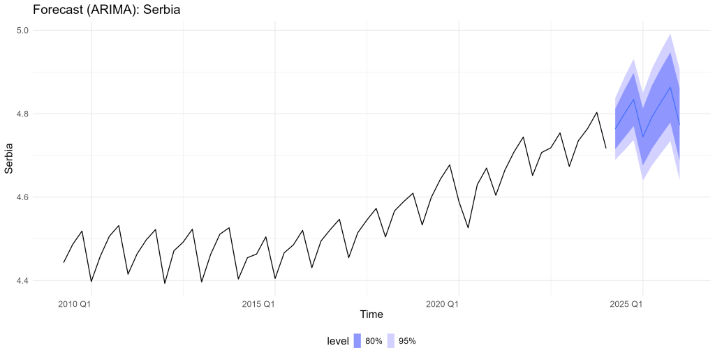
Several point forecasts are very close to the observed values. In 2024Q3, for example, the actual value is 121.377 and the forecast mean is 121.470. In 2024Q4, the actual value is 126.114 and the forecast mean is 125.726. In other quarters, the forecast is less exact but still close in relation to the level of the GDP index. The model slightly underestimates some observations and slightly overestimates others, but there is no obvious pattern of persistent overprediction or underprediction across the holdout period.
Table 3. Forecast eight quarters ahead — ARIMA model
| Date | Actual | Mean | Lower 80% | Upper 80% | Lower 95% | Upper 95% |
|---|---|---|---|---|---|---|
| 2024 Q2 | 118.9 | 117.1 | 111.6 | 122.9 | 108.8 | 126.1 |
| 2024 Q3 | 121.4 | 121.5 | 114.7 | 128.6 | 111.3 | 132.6 |
| 2024 Q4 | 126.1 | 125.7 | 118.0 | 134.0 | 114.1 | 138.6 |
| 2025 Q1 | 113.9 | 114.9 | 107.3 | 123.1 | 103.5 | 127.6 |
| 2025 Q2 | 121.4 | 120.5 | 111.7 | 130.0 | 107.4 | 135.4 |
| 2025 Q3 | 123.8 | 125.0 | 115.4 | 135.5 | 110.6 | 141.4 |
| 2025 Q4 | 128.9 | 129.4 | 119.0 | 140.8 | 113.8 | 147.2 |
| 2026 Q1 | 117.6 | 118.3 | 108.4 | 129.1 | 103.5 | 135.2 |
The forecast should be interpreted as a baseline statistical projection rather than a full macroeconomic scenario. It is useful precisely because it provides a disciplined benchmark: if the actual GDP series moves far outside the forecast interval, that would be a warning sign that new information has entered the system. However, the model does not know in advance about future policy shocks, energy-price shocks, geopolitical changes or sudden changes in external demand. It will recognise such developments only after they appear in the data.
The conclusion from Part 2 is therefore positive but cautious. The ARIMA model captures Serbia’s short-term GDP dynamics well over the holdout period. It is useful for monitoring and near-term projection, but it should be combined with economic judgement and contextual information when used for policy analysis or public commentary.
Methodological appendix to Part 2
ARIMA stands for autoregressive integrated moving average. “Autoregressive” means that current values depend partly on past values. “Integrated” means that differencing is used to make a non-stationary series more suitable for modelling. “Moving average” means that current values also depend on past forecast errors or innovations. Seasonal ARIMA models extend this logic to regular seasonal patterns, which is especially relevant for quarterly GDP. In this analysis, the sample is divided into a training period and an eight-quarter holdout period. The model is estimated on the training part and then used to forecast the holdout observations. This separation is important because a model can fit the past well and still forecast poorly. Forecast accuracy is assessed using measures such as RMSE, MAE and MAPE. RMSE gives more weight to larger errors, MAE measures average absolute error and MAPE expresses error as a percentage of the observed values. Residual diagnostics, including the Ljung-Box test, check whether the model has left systematic autocorrelation unexplained.